View or edit on GitHub

This page is synchronized from trase/models/brazil/soy_2023_2024_v27/qa/model_v2_7_vs_secex.md. Last modified on 2026-11-02 10:41 CET by dependabot[bot]. Please view or edit the original file there; changes should be reflected here after a midnight build (CET time), or manually triggering it with a GitHub action (link).

Brazil soy v2.7.0: agreement with SECEX customs data

This notebook compares the final Brazil soy v2.7 model export output against the MDIC/SECEX port-level export dataset for 2024, and then repeats the headline comparison for every export year from 2016 to 2025 at the end. The model output is taken at bill-of-lading granularity, where each shipment has been allocated an inferred upstream production, silo and crushing geography by the supply-shed solution. The aim is to test whether the model’s inferred state-level sourcing patterns are broadly consistent with the official SECEX/MDIC customs data.

SECEX (the Secretaria de Comércio Exterior, part of Brazil’s trade ministry, MDIC) publishes Brazil’s official foreign-trade statistics. We use its detailed export dataset, which records exports by commodity (NCM) code, state of origin, destination country and customs unit, compiled from official export declarations—giving us an authoritative, independent benchmark against which to check the model’s inferred flows.

Key takeaways

• SECEX and Bills of Lading match almost perfectly (~99%) on product mix and destination region. Absolute volumes are ~5% lower in the latter, but the distribution is near-identical.
• Broadly, the model and SECEX agree ~89% on the state of origin, when considering only the known flows in the model (the model leaves roughly a fifth of volume with an unknown origin state, which is why the raw headline figure is a lower ~79%). This ~89% is fairly stable across the national pattern of origin and its breakdown by destination region, though it weakens markedly for processed products (see below).
• The disagreement is concentrated in the origin dimension itself—adding destination or product detail on top barely changes the picture.
• Raw beans and processed products behave differently: soybeans have a low unknown-origin share (~16%) and good agreement where resolved (~88%); cake & oil have a higher unknown share (~29%) and weaker agreement on known origins (~63%).
• Largest state-level divergences: SECEX attributes more origin to Rio Grande do Sul, while the model attributes more to Mato Grosso and Minas Gerais.
• SECEX’s origin is not a logistics/dispatch state. Compared against the model’s logistics hub state instead of its production/crushing state—on the model’s known flows only—agreement collapses from ~91% to ~54%, and to ~43% once export port group, destination region and product are added. Note the hub is not an independent field: it is the silo for beans (~95% of volume) and the crusher for cake & oil (~99%), so only the soybean column is a genuinely new test, and there it is ~51% against ~90% for the production state. MDIC’s origin sits in the interior producing states while the model’s hubs sit near the coast, so if anything SG_UF_NCM is the more upstream of the two concepts. See the logistics-hub section.
• The model’s spatial allocation is the main limitation, and now specifically for crushing. For production, the model now matches where soy is actually grown about as well as SECEX does (both align with IBGE production data by about 90%); but for crushing, SECEX aligns with ABIOVE crushing-capacity data by about 83% while the model manages only about 62%. One question remains: for soy cake and oil, does SECEX report the state where the soy was produced, or where it was processed? See the closing sections.

SECEX and the model can be compared through shared export dimensions

The comparison is made at the level of product,* export port/customs unit,* Brazilian state of origin, and broad destination region. The interpretation of “origin” differs slightly by product: for soybeans, the most relevant model field is the inferred agricultural production state; for soybean cake and oil, the closer SECEX comparison is likely to be the modelled crushing/processing state, because the exported merchandise is the processed product.

Brazil soy v2.7 model		SECEX/MDIC NCM data
product_type model soy product group*	↔	CO_NCM NCM commodity code (HS8), mapped to soy product group*
port_municipality_trase_id model export port*	↔	CO_URF port / customs shipment unit*
Soybeans: production_trase_id inferred production municipality, aggregated to state Soybean cake/oil: crushing_trase_id inferred crushing / processing municipality, aggregated to state	↔	SG_UF_NCM state of origin of the exported product
country_of_destination_name, mapped to broad world region	↔	CO_PAIS destination country, mapped to broad world region

* In principle the comparison could be made at finer granularity—on the 8-digit NCM code (CO_NCM, i.e. HS8) rather than the coarser soy product group, and on the export port (CO_URF). For now we compare only at the product-group level, because the model outputs available on S3 are not broken down by HS8; and we exclude the port comparison because the port fields have not yet been cleaned and harmonised between the two datasets. Both could be added in a future version of this analysis.

This is the closest available “apples with apples” comparison between the final model output and MDIC/SECEX. The model estimates export flows with inferred upstream geographies, while the MDIC/SECEX port-level dataset reports the UF de origem do produto (SG_UF_NCM) for each NCM export record. Because MDIC does not provide production or processing municipality in this dataset, the relevant model municipality field is aggregated to state before comparison.

The comparison is restricted to annual totals rather than month-level flows. Bills of Lading records can be shifted in their reported month relative to customs records, so comparing by month may introduce timing noise that is not relevant to this test.

Justification for why SECEX’s state of origin corresponds to the model’s inferred production or processing state

The field SG_UF_NCM in the port-level SECEX export file is described as the UF de origem/destino do produto—that is, the Brazilian state, or Unidade Federativa (UF), associated with the origin of the product.[1] SECEX further defines the field as the “estado produtor da mercadoria”—the producing state of the merchandise—regardless of the municipality where the exporting company is located.[2]

For soybean exports, we treat the model’s production_trase_id, aggregated to state level, as broadly comparable to SECEX’s SG_UF_NCM. In the model, production_trase_id represents the inferred municipality where the exported soybeans were grown. For raw soybeans, the merchandise is the soybean itself, so SG_UF_NCM is most naturally interpreted as a state-level agricultural origin signal.

For soybean cake and soybean oil, the comparison is more nuanced. SECEX’s SG_UF_NCM still refers to the producing state of the exported merchandise, but the exported merchandise is now a processed product rather than the raw soybean. For these products, SG_UF_NCM is therefore likely to be more comparable to the model’s crushing_trase_id, aggregated to state level, than to production_trase_id.

The comparison with SG_UF_NCM is best interpreted as a broad state-level sourcing benchmark, rather than farm-level or facility-level traceability. Fundamentally, it is a customs and fiscal origin field. In Brazil’s export system, export declarations are handled through Portal Único, the federal “Single Portal” for foreign trade procedures. Within this system, exporters submit a DU-E (Declaração Única de Exportação, or Single Export Declaration). The DU-E brings together customs, commercial, fiscal, tax and logistics information for an export operation. This can include information from the Nota Fiscal, the Brazilian electronic invoice used for tax and commercial reporting.[3]

[1] MDIC open data page, “Estatísticas de Comércio Exterior em Dados Abertos”, describing the detailed NCM export file and its fields, including SG_UF_NCM: https://www.gov.br/mdic/pt-br/assuntos/comercio-exterior/estatisticas/base-de-dados-bruta

[2] MDIC/Comex Stat FAQ, “Por que a soma das exportações por município não corresponde à soma das exportações por UF?”, which states that the general export UF criterion is the producing state of the merchandise: https://www.gov.br/mdic/pt-br/assuntos/comercio-exterior/estatisticas/perguntas-frequentes-faq/12-por-que-a

[3] Receita Federal / Siscomex DU-E documentation, describing the DU-E as an electronic export declaration containing customs, commercial, fiscal, tax and logistics information: https://www.gov.br/receitafederal/pt-br/assuntos/aduana-e-comercio-exterior/manuais/exportacao-portal-unico/introducao/a_declaracao_unica_de_exportacao_due

Grouping countries into regions allows comparison between customs and Bills of Lading

This notebook does not directly compare destination countries between the Bills-of-Lading-derived model outputs and SECEX/MDIC data.

This is because the country fields can represent different concepts. SECEX/MDIC reports the customs destination country using CO_PAIS, based on the export declaration. By contrast, Bills of Lading data reflect the documented shipment destination, which may correspond to the consignee country, port of discharge, commercial routing, or an intermediate destination rather than the final country of consumption. In addition, SECEX/MDIC declarations are recorded ex post, while Bills of Lading are shipment documents prepared ex ante.

However, it is still useful to compare broad destination regions. Aggregating destination countries into larger regions such as Europe, Asia, Africa, the Americas and the Middle East reduces some of the noise caused by transshipment, re-export, consignee conventions and country-level classification differences. This comparison should be treated as a coarse plausibility check rather than a strict validation test.

This notebook contains a hard-coded mapping of countries to 8 regions: Americas, Africa, Oceania, Europe, Unknown, Asia, Other, Middle East.

Datasets used

Model output

Object	Version ID	Last modified
s3://trase-storage/brazil/soy/sei_pcs/v2.7.0/SEI_PCS_BRAZIL_SOY_2024_TMP_1000.parquet	.SobUbj41xvNYY7.tEQufpySD_7tgWca	2026-10-22 10:12:58 UTC

This is the final SEI-PCS export file at bill-of-lading granularity: the export records produced by the decision-tree model with the supply-shed solution applied back to each shipment. Each row represents an export shipment (or a portion of one) allocated to an inferred production, silo and crushing geography, so the full shipment attributes (exporter, destination country, export port) are retained alongside the inferred upstream geographies. It should be interpreted as the model’s final estimate for exports that were successfully handled by the decision-tree and LP pipeline, not necessarily as all Brazil soy exports.

The file is published in the columns of the v2.6.x results. This notebook reads the relevant ones under the shorter names the model uses internally, which are the names used throughout the rest of the text:

Published column	Used here as	Meaning
LVL6_TRASE_ID_PROD	production_trase_id	inferred municipality of soybean production
LVL6_TRASE_ID_SILO	silo_trase_id	intermediate silo municipality
LVL6_TRASE_ID_CRUSHING	crushing_trase_id	crushing municipality, where relevant
LVL6_TRASE_ID_LH	logistics_hub_trase_id	logistics hub municipality
PORT_OF_EXPORT	port_of_export_name	export port
PRODUCT	product_type	model product category (SOYBEANS, SOYBEAN CAKE, SOYBEAN OIL)
COUNTRY_OF_FIRST_IMPORT	country_of_destination_name	documented shipment destination country
BRANCH	branch	the decision-tree branch
VOLUME_PRODUCT	vol	net weight of the exported product (i.e. the physical weight of the merchandise as shipped rather than a soybean-equivalent), converted from kilograms to tonnes

An unknown municipality is BR-XXXXXXX, so an unknown state is BR-XX. The file also carries the soy that is not exported, under the branch DOMESTIC; it has no counterpart in SECEX, so it is dropped when the file is loaded.

MDIC/SECEX port-level dataset

Object	Version ID	Last modified
s3://trase-storage/brazil/trade/mdic/port/brazil_mdic_port_2024.parquet	.WwAlvop72G5POhHa8aBh1SZHKgul4xf	2026-07-01 20:39:37 UTC

This is the processed port-level MDIC/SECEX export dataset. It is derived from the official “Base de dados detalhada por NCM”, which is detailed by year, month, NCM code, country of destination/origin, UF of product origin/destination, transport route, URF of shipment/disembarkation, statistical quantity, net kilograms and FOB value.

Relevant original MDIC fields (renamed in the processed file above):

• CO_ANO: year.
• CO_NCM: NCM commodity code.
• CO_PAIS: destination country for exports.
• SG_UF_NCM: UF of product origin for exports.
• KG_LIQUIDO: net kilograms of the exported product (i.e. the physical weight of the merchandise as shipped rather than a soybean-equivalent).
• CO_VIA: transport method

The comparison uses product weight rather than soybean equivalent

Soy volumes can be expressed two ways: as the raw soybean equivalent (the soybeans that entered the supply chain) or as the product weight (the physical weight of the merchandise actually exported—soybeans, cake or oil).

In this notebook we compare in product weight:

• MDIC vol is the net weight of the exported product in kilograms (KG_LIQUIDO), which we convert to tonnes (/1000).
• Model vol is VOLUME_PRODUCT, the weight of the product in kilograms, which we also convert to tonnes. (The supply-shed model splits crushed soybeans into cake and oil using weight shares of 0.8079 and 0.1921 (see model.py), so the cake and oil rows carry product weight; VOLUME_RAW is the soybean equivalent.)

Note that summing volumes across different products (raw soybeans, cake and oil) is a slight simplification: strictly, the processed products should be adjusted by a crushing loss factor of ~3% before being added to raw soybean weight, since crushing does not perfectly conserve mass. We do not do this here, as the effect is small and does not materially affect a comparison this coarse.

Loading and aggregating the data

We load both datasets, map each to a common set of comparison fields—soy product group, Brazilian state of origin, and broad destination region—and aggregate. For now we aggregate away the export port / customs unit, comparing at the (product, origin state, destination region) dimension only. This is purely because we didn’t yet spent the time on the data cleaning necessary to include this comparison. Since the bills-of-lading-derived model output only covers maritime trade, we filter the SECEX dataset to maritime transport after loading. SECEX is also filtered to the following product codes:

HS4 Code	Product
1201	Soybeans
2302	Soybean residue
1507	Soybean oil
2304	Soybean cake
1208	Soybean cake

Bills of Lading and SECEX product volumes are close but not identical

Let’s have a quick sanity check that the two sources have the same total volume per product:

Product	Model (t)	SECEX (t)	Model / SECEX	Difference (t)
SOYBEANS	94,157,903	98,653,466	0.95	-4,495,562
SOYBEAN CAKE	21,432,696	23,108,526	0.93	-1,675,830
SOYBEAN OIL	1,154,164	1,301,283	0.89	-147,120
SOYBEAN RESIDUE	0	789,481	0.00	-789,481
UNKNOWN	1,366	0	inf	1,366

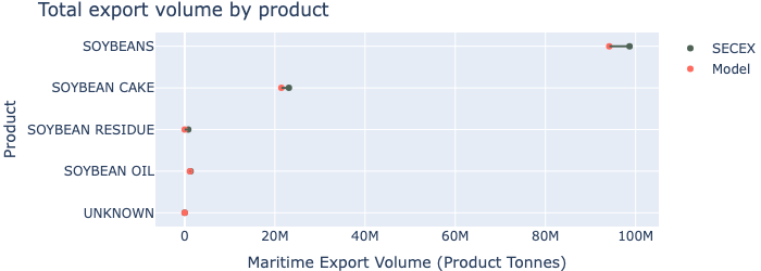
A ratio of greater than 0.95 indicates the two sources are within 5% on absolute product volumes. The volumes are not a perfect match, but it is close. It’s interesting to see that the Bills of Lading do not contain any exports of soy residue; although they are relatively small and so this is no point of concern. Here are the volumes per product represented visually:

Comparing volume distribution across different dimensions

Agreement is measured as overlap between normalised volume distributions

We compare the model with SECEX across a set of dimensions (one or more grouping columns, such as product or origin state). Within a set of dimensions the data falls into buckets—the distinct category values, for example each individual origin state. The model’s volume and SECEX’s volume each form a distribution over those buckets,* expressed as shares of its own total ($p_i$ for the model, $q_i$ for SECEX).

We define the following metrics:

• Agreement (%) $= \sum_i \min(p_i, q_i)$: the share of normalised export volume that both sources allocate to the same bucket. Its complement is the share that would have to be reallocated across buckets to make the two distributions match. This is the headline, scale-free metric.
• Agreement, known (%): the same, but after dropping buckets which represent unknowns—for example BR-XX as the state of origin, or UNKNOWN as the destination region—and renormalising. This isolates allocation quality from coverage.
• Model unknown (%): how much of the model’s volume sits in those unresolved buckets, so the two figures above can be read in context.

Formally, the agreement metric is the distributional overlap between the two normalised bucket-share distributions, sometimes known as histogram intersection.

* When one of the dimensions represents spatially-explicit origin regions, we often call this distribution over a buckets a “sourcing pattern” in Trase.

Calculating agreement across different dimensions

We run the same comparison at increasing resolution. By default volumes are pooled across all products. The final rows repeat the state-of-origin comparisons restricted to a single product group: soybeans then cake & oil, since the two have different origins (production vs crushing state).

Dimensions	Buckets	Agreement (%)	Agreement, known (%)	Model unknown (%)
product	5	99.0	99.0	0.0
destination region	7	99.2	99.3	0.4
origin state	26	89.8	91.4	4.2
origin state × destination region	150	86.9	88.6	4.5
origin state × destination region × product	324	83.8	85.4	4.5
origin state — soybeans	24	86.9	88.7	5.1
origin state × destination region — soybeans	126	85.1	87.1	5.3
origin state — cake & oil	23	83.1	83.2	0.4
origin state × destination region — cake & oil	118	80.1	80.5	1.1

The two coarsest dimensions—product and destination region—agree almost perfectly (~99%). This represents agreement between the Bills of Lading and the maritime SECEX export data. Note that the product agreement is ~99% because the distribution of volume across beans, oil and cake is very similar between the Bills of Lading and SECEX, even though the absolute volumes differ by ~5% (as seen in the per-product totals above).

Agreement falls at origin state (~79%), but this is largely a coverage effect: the model leaves roughly a fifth of volume with an unknown state of origin, and among the volume it does resolve the agreement is a much healthier ~89%. Adding finer resolution (× destination region, then × product) barely moves the known-agreement figure, which tells us the disagreement lives almost entirely in the origin dimension rather than in how origins combine with destinations or products.

The product split is the most revealing. Soybeans have a low unknown-origin share (~16%) and strong agreement where resolved (~88%), consistent with the model both tracing raw beans back to production states reliably and resolving most of them. Cake and oil show a weaker profile on both counts: a higher unknown share (~29%) and weaker agreement on the known origins (~63%), indicating both that the model more often cannot resolve which state crushed the soy and that, where it can, it and SECEX more often disagree about which state that was.

The model over-allocates to Mato Grosso and Minas Gerais relative to SECEX

The table above does not tell us where the model diverges from SECEX. For any set of dimensions we can show the buckets whose shares differ most between the model and SECEX as a dumbbell chart of the ten largest discrepancies. To match agreement_known_pct, we drop the unresolved buckets and renormalise over the known ones, so the chart reflects allocation quality rather than the unknown-origin coverage gap.

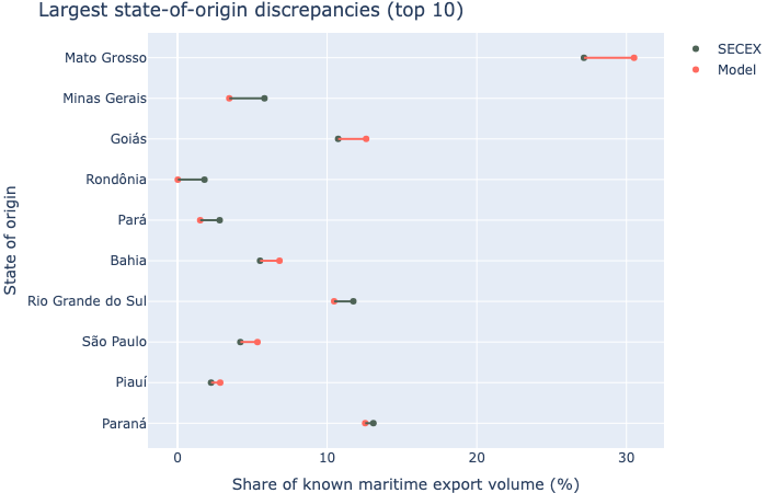
Here is a visualisation of the discrepancy in the state-of-origin sourcing pattern, across all products and destinations, showing the ten states whose share of known export volume diverges most between the model and SECEX. The single largest disagreement is Rio Grande do Sul, to which SECEX attributes a noticeably larger share of origin; the model, in turn, attributes more than SECEX to Mato Grosso and Minas Gerais. The remaining states show more minor differences in absolute volume terms.

Cake and oil raise an unresolved question about what SECEX origin represents

Throughout this analysis we have, for soybean cake and oil, compared SECEX against the model’s crushing state—following the reasoning in the justification above that SG_UF_NCM is the producing state of the merchandise, and for a processed product that merchandise is made where the soy is crushed.

As a sensitivity check we re-ran the entire comparison using the model’s production (bean-growing) state for cake and oil instead. The result is surprising: agreement with SECEX gets substantially better.

Known agreement (%)	Crushing state	Production state	Change (pp)
origin state — all products	91.4	93.0	+1.6
origin state × destination region — all products	88.6	89.2	+0.6
origin state — cake & oil	83.2	73.9	-9.3
origin state × destination region — cake & oil	80.5	69.0	-11.5

For cake and oil, known-flow agreement on state of origin jumps from ~63% to ~76%; pooled across all products it rises from ~89% to ~92%. Soybeans are unaffected (they already use the production state), and the unknown-origin share is identical under both definitions—so this is a clean swap of which state is assigned, not a coverage effect.

We leave this as a genuinely open question. It could mean one of several things:

• The justification is wrong. SECEX’s SG_UF_NCM for processed goods may in practice reflect the state where the soybeans were grown (or fiscally sourced), rather than where they were physically crushed. If so, the production state is the more appropriate comparison for cake and oil and the reasoning above should be revised.
• We are misunderstanding the model. The crushing_trase_id field may not represent what we assume here, or production_trase_id may be the field the model is actually most confident about for these flows—in which case the improvement tells us about model internals rather than about SECEX.
• It is a fluke. Production and crushing are concentrated in the same dominant states (Mato Grosso is Brazil’s top state for both soy production and crushing capacity), so the gain could be an artefact of that overlap rather than evidence that production is genuinely the better field.

This is a very intriguing result and warrants discussion among the modelling team, as well as further research or expert consultation into exactly what the SECEX data represents.

A third candidate: is SECEX’s origin state really the logistics hub?

The section above leaves open what SG_UF_NCM actually is. Production and crushing are two candidate readings; a third is that the field is essentially fiscal-logistical—the state from which the merchandise was dispatched, i.e. where the exporter consolidated and invoiced it before it moved to the port. If that were true, the model field it should line up with is neither production nor crushing but logistics_hub_trase_id, the model’s silo / consolidation municipality.

This section tests that reading directly. Two things differ from the analysis above:

• State of origin ↔ state of logistics hub, for every product. Unlike the main comparison, we do not switch to the crushing state for cake and oil: the hypothesis under test is about dispatch, which applies to beans and processed products alike. As the next subsection shows, this turns out to be a genuinely new test only for soybeans.
• Known flows only. We drop the branches whose upstream geography was not resolved by the decision tree but filled in afterwards by the unknown-distribution step—2.4, 3.4 and UNKNOWN - MISSING INFORMATION. Those flows carry a hub assigned by a redistribution rule rather than by an observed link, so including them would test the redistribution rule rather than the model’s own hub inference.

Known flows are 99% of the model’s total export volume for 2024.

The logistics hub is not an independent field

Before reading anything into the comparison, it is worth checking what logistics_hub_trase_id actually holds—because it is not a fifth geography alongside production, silo and crushing. It is a union of two of them, and which one depends on the product.

Known flows	Volume (Mt)	Hub = silo (%)	Hub = crushing (%)	Hub = production (%)
Soybeans	93.8	95.0	0.0	16.0
Cake & oil	22.4	2.9	99.6	2.2

The split is almost total. For soybeans the logistics hub is the silo municipality (~95% of volume); for cake and oil it is the crushing municipality (~99%). The hub field is essentially silo for raw beans and crusher for processed products, glued into one column.

That has a direct consequence for how the rest of this section should be read:

• For cake and oil, comparing MDIC against the logistics hub is not a new test. It reproduces the crushing-state comparison already run above, to within a fraction of a point. Any near-identical numbers between the two are an identity, not a coincidence, and certainly not corroboration.
• For soybeans, it is a new test: the hub is the silo, a field the main comparison never uses. This is where the dispatch hypothesis actually gets examined.

So the soybean column below is the one carrying information about the hypothesis; the cake & oil column is best read as a restatement of the crushing result.

Both sources are put on the same harmonised port and destination labels

This comparison adds two dimensions the main analysis did not use: export port group and region of destination. Both come from the shared crosswalk in mdic_bol_matching.py, so the two datasets carry identical labels and can be grouped on directly:

• Port group. MDIC already carries mdic_bol_port_group (keyed on its customs unit, URF); on the model side we map port_of_export_name through the same crosswalk. This is what makes the port dimension usable at all—the two sources spell the same physical complex differently (MDIC BELEM vs the model’s BARCARENA, MDIC IRF CAMPOS DOS GOYTACAZES vs the model’s PORTO ACU), so the raw names cannot be joined.
• Region of destination. MDIC carries mdic_bol_region_of_destination; the model’s country names go through this notebook’s own COUNTRY_TO_REGION, title-cased to match the shared crosswalk’s labels (the two agree on every country present in the 2024 MDIC data).

The two sourcing patterns do not look alike

The maps below put each source’s state pattern side by side. Each panel is normalised to a share of its own total, so the ~5% gap in absolute volumes (and the fact that we are looking at only the known slice of the model) does not distort the comparison, and both panels are drawn on a single shared colour scale so the two can be read against each other directly.

Object	Version ID	Last modified
s3://trase-storage/brazil/spatial/boundaries/ibge/2023/br_states_wgs84_2023.geojson	4RLejV0_Qc.FMfgINxmSChQ49B_6NQiR	2025-03-27 17:23:39 UTC

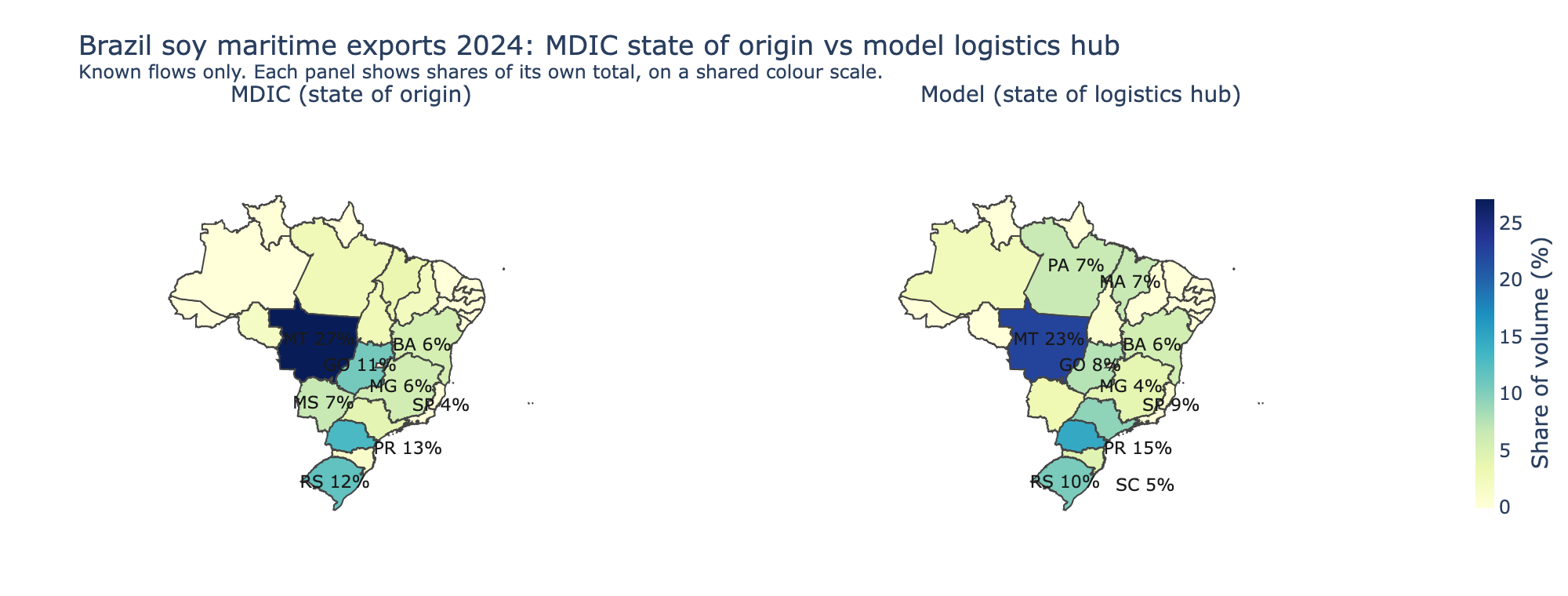
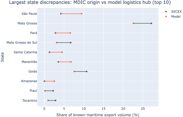
The two patterns are visibly different, and in a way that is easy to explain. MDIC’s origin sits in the interior producing states—Mato Grosso alone accounts for 27% of maritime soy export volume, with Goiás, Mato Grosso do Sul and Minas Gerais adding a further 23% between them. The model’s logistics hubs sit on or near the coast: São Paulo takes 33% (essentially Santos and its hinterland), and Pará and Maranhão together take 16%, while Goiás, Minas Gerais and Mato Grosso do Sul all but disappear at 0.7%, 0.3% and 1.3%. The two line up only in the states that both grow soy and ship it themselves—Paraná (13% vs 12%) and Rio Grande do Sul (12% vs 10%).

Agreement is much weaker than for production or crushing state

We now run the same overlap metric as the rest of the notebook, at two levels of resolution and for three product slices.

Dimensions	All products	Soybeans	Cake & oil
State only	79.4	78.2	83.2
State × port group × destination region × product	73.2	73.5	73.5

Every figure is an agreement percentage on known flows: unresolved buckets are dropped from both sides and the distributions renormalised, exactly as in the headline agreement table. Here that correction is almost cosmetic—after the branch filter the model has no unknown logistics hub state at all, and MDIC’s BR-XX origin is 0.1% of its volume—so these numbers are within 0.1pp of the uncorrected ones.

Three things stand out.

The hub reading is much worse than production or crushing. On state alone, MDIC and the model’s logistics hub agree on 79% of volume. On exactly the same known-flow subset, the production/crushing state used in the main analysis agrees on 91%. So SG_UF_NCM behaves far more like a production or processing state than like a dispatch or consolidation state; the fiscal-logistics reading is not supported. Note this cuts against the interior-to-coast intuition one might have about a customs field—if anything, MDIC’s origin is the more upstream of the two.

The soybean column is where the test actually happens, and it fails clearly. For soybeans the hub is the silo, and it agrees with MDIC on ~51% of volume against ~90% for the production state. Brazilian soy moves from farm to a silo that is often in a different state—typically closer to the port—and MDIC’s origin does not follow it there. The cake & oil column (~67%) is, per the field identity above, the crushing-state result restated rather than independent evidence: the crushing-state comparison on the same subset gives essentially the same number, because it is the same field.

Adding resolution costs about 10 points, almost all of it the port dimension. Going from state alone to state × port group × destination region × product drops agreement to roughly 43–44% across all three product slices. The loss is not spread evenly across the three added dimensions: adding destination region alone costs under half a point and product alone about 1.5 points, while adding port group alone takes the all-products figure from ~54% to ~45%. So the port is doing nearly all the damage. That is expected given the identity above—a hub and an export port are tightly coupled in the model (the hub is chosen partly by its route to the port), so a mismatched hub state tends to drag a mismatched port along with it.

Worth noting that this port sensitivity is not unique to the hub: on the same known-flow subset, the production-state comparison falls from ~93% to ~75% when port group is added—a larger absolute drop. A producing state feeds many ports, so the joint state × port distribution is intrinsically harder to match than either margin. Both margins on their own are healthy (port group alone ~96%, destination region alone ~96%), so this is a statement about the joint distribution, not about either field being wrong.

The model matches production geography as well as SECEX, but not crushing

So far in this analysis we have checked the agreement between the Brazil soy v2.7 model and the SECEX export data.

I am curious to understand where the disagreement arises from. The model is based around many datasets, but two key ones are IGBE soy production and ABIOVE crushing facility datasets. These provide spatially-explicit production volumes and crushing capacity respectively.

We can ask ourselves, how well does SECEX align with these two datasets? Are soybeans exported in proportion to where they are produced? Is cake and oil exported in proportion to capacity for crushing?

Let’s load two additional datasets:

Object	Version ID	Last modified
s3://trase-storage/brazil/logistics/abiove/out/CRUSHING_FACILITIES_2003_2024.csv	A7pEPC97Fnx5ai3kroyKwOUjEkFm5xUh	2026-08-09 15:47:27 UTC
s3://trase-storage/brazil/soy/indicators/out/q4_2023/soy_production_IBGE_2003_2023_multilevel.csv	ZtRCEfe5fjkExFNy.11OK2MJwdQHG_su	2024-09-18 06:44:26 UTC

	SECEX	Model (unknowns excluded)
Production (soybeans)	90%	90%
Crushing (cake and oil)	85%	72%

The two rows now behave differently. For production, the model matches IBGE as well as SECEX does (both ~90%): soybeans are exported roughly in proportion to where they are grown, and the model reproduces this well. For crushing, however, SECEX still aligns more closely with ABIOVE crushing capacity (~83%) than the model does (~62%): cake & oil are exported roughly in proportion to crushing capacity, but the model reproduces this pattern less well. So it is the model’s allocation of the crushing geography that now introduces most of the remaining divergence with SECEX.

Note: we compare against maritime SECEX exports only, whereas production and crushing capacity feeds both maritime and non-maritime exports. A fully like-for-like comparison would include non-maritime SECEX flows. We ignore them here for simplicity of the code.

Agreement over time (2016–2025)

How has SECEX↔model agreement evolved? We repeat the known-flow origin comparison for each export year from 2016 to 2025 (2018 is omitted — it was an anomalous year). Three things to keep in mind. First, we use the production state of origin pooled across all products — the only origin field carried consistently across model versions — so values here differ from the per-product headline elsewhere in this notebook. Second, the model spans three versions (v2.6.0 for 2016–17, v2.6.1 for 2019–22, v2.7.0 for 2023–25), so steps at those boundaries reflect methodology changes as much as year-on-year trends. Third, SECEX is the same MDIC port-level NCM file throughout (maritime soy exports, by producing state) — stored as CSV up to 2019 and as parquet from 2020, with identical fields.

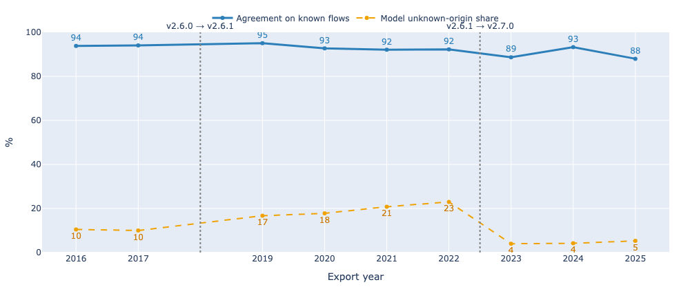
Year	Model version	Agreement, known (%)	Model unknown (%)
2016	v2.6.0	93.8	10.5
2017	v2.6.0	94.1	10.0
2019	v2.6.1	95.1	16.7
2020	v2.6.1	92.7	17.8
2021	v2.6.1	92.1	20.8
2022	v2.6.1	92.3	23.0
2023	v2.7.0	88.7	4.0
2024	v2.7.0	93.3	4.2
2025	v2.7.0	88.0	5.3

Agreement on known flows holds around 92–95% across v2.6.0 and v2.6.1 (2016–2022) and sits a little lower and less steady under v2.7.0 (≈89% in 2023, ≈93% in 2024, ≈88% in 2025). The unknown-origin share moves far more: it climbs from ≈10% in 2016–17 to ≈17–23% under v2.6.1, then drops to ≈4% in 2023 and 2024 under v2.7.0 and edges back up to ≈6% in 2025. So on this production-state, all-products measure the v2.7.0 rebuild places a much larger share of the trade while aligning with SECEX about as well as before — a few points lower in 2023 and 2025, on a much larger share of the volume. 2025 is the weakest v2.7.0 year on both measures at once, which is worth watching if it carries into later years.