View or edit on GitHub
This page is synchronized from trase/products/analysis/notebooks/qa/brazil_soy_2023_24/unknown_allocation_method_comparison.md. Last modified on 2026-09-20 13:50 CEST by Nicolas Martin.
Please view or edit the original file there; changes should be reflected here after a midnight build (CET time),
or manually triggering it with a GitHub action (link).
Brazil soy v2.7: Comparing unknown-flow allocation methods (2023)
The soy v2.7 model offers two ways to redistribute unknown-origin flows:
alloc_unknowns_by_known_pattern (based on observed market behaviour,
via MDIC state distributions) and alloc_unknowns_by_facility_capacity
(based on soy facility capacity). See
readme_unknown_allocation.md
for the full methodology and the ab_test_s3.py workflow used to
produce the two runs compared here.
This notebook loads the final SEI-PCS export file (bill-of-lading granularity, year 2023) produced by each method and compares some headline numbers.
Datasets used
| Object | Version ID | Last modified |
|---|---|---|
s3://trase-storage/brazil/soy/sei_pcs/v2.7.0/_ab_test/pattern/SEI_PCS_BRAZIL_SOY_2023_TMP_1000.parquet |
DlrRzjJZ0SaLLRy8531yWYaNOI5E_DAj | 2026-08-18 13:11:35 UTC |
s3://trase-storage/brazil/soy/sei_pcs/v2.7.0/_ab_test/capacity/SEI_PCS_BRAZIL_SOY_2023_TMP_1000.parquet |
WDVALwu4Ts4W37hDTa0j0At0uhKRijlZ | 2026-08-18 13:27:58 UTC |
These are backups of the final SEI-PCS export file at bill-of-lading
granularity, taken via ab_test_s3.py backup right after a full run of
main.py for each allocation method — see the runbook in the
readme
on #5598.
Headline comparison
In the below metric:
- Unknown branch volume is the amount of volume that is left in the “unknown” branch, (called “UNKNOWN - MISSING INFORMATION”).
- Unknown production volume is the amount of volume for which the production region is unknown
The data in this table comes from the total export records - i.e. all branches included.
| Method | Rows | Unknown branch volume % | Unknown production volume % | Distinct logistics hub municipalities | Distinct logistics hub states |
|---|---|---|---|---|---|
| Known market pattern | 648,177 | 0.47 | 3.86 | 127 | 17 |
| Facility capacity | 1,900,209 | 0.64 | 79.28 | 1,481 | 19 |
We see that the facility capacity method has about 3x the row count and has 11x the number of distinct logistic hub municipalities.
How close are the two runs, outside the geographical allocation itself?
The two methods only differ in how they assign upstream geography
(logistics_hub_trase_id, production_trase_id, silo_trase_id,
crushing_trase_id) to previously-unknown flows, and in how much of
that volume they manage to resolve at all. Rather than a pass/fail test,
this section asks how close the two runs are on everything else, at
two different levels of strictness, and reports the distribution of
differences rather than collapsing it to a single verdict — a fixed
tolerance either drowns in noise from trivially small groups or has to
be tuned against the very data it’s checking.
Before comparing how volume is grouped, it’s worth checking whether there’s even the same amount of it to begin with:
Summed across the entire export file:
- Volume: 116,366,730.02 t (pattern) vs 116,366,729.98 t (capacity) — 0.000000% apart.
- FOB: \$99,783,321,696.97 (pattern) vs \$99,783,321,668.85 (capacity) — 0.00000003% apart.
Both are floating-point-summation-noise scale, not a real discrepancy: the two runs are redistributing the same pool of volume and value. Everything below is entirely about how that pool gets grouped, not about how much of it exists.
Column check: every column is accounted for (grouped on, or expected to be ignored).
Comparison 1: the whole export file, trade data only
Every row from both runs, every branch included — geography (branch,
logistics_hub_trase_id, and everything downstream of it) dropped
entirely, leaving only the trade-data columns a change of allocation
method should never touch.
All 648,177 (pattern) / 1,900,209 (capacity) rows, grouped by
country_of_destination_name, exporter_cnpj, exporter_cnpj8,
exporter_group, exporter_label, exporter_name,
port_municipality_trase_id, port_of_export_label,
port_of_export_name, product_type, year — 1,933 groups.
| Metric | P50 | P75 | P90 | P100 (max) |
|---|---|---|---|---|
| Volume — absolute diff | 0.0 t | 0.0 t | 0.0 t | 0.0 t |
| Volume — relative diff | 0.0% | 0.0% | 0.0% | 0.0% |
| FOB — absolute diff | \$0 | \$0 | \$0 | \$4 |
| FOB — relative diff | 0.0% | 0.0% | 0.0% | 0.0% |
Comparison 2: branches untouched by the allocation method, trade data + logistics hub
Only rows whose branch isn’t produced or renamed by the unknown-flow
allocation step — for these, logistics_hub_trase_id is set by the
decision tree, not by the allocation method, so it’s added to the
grouping key as a stricter check on top of Comparison 1.
All rows except branch 2.4 DISTRIBUTION OF UNKNOWNS,
2.4 DISTRIBUTION OF UNKNOWNS BY CAPACITY,
3.4 DISTRIBUTION OF UNKNOWNS, UNKNOWN - MISSING INFORMATION — 78,521
(pattern) / 30,195 (capacity) rows, grouped by
country_of_destination_name, exporter_cnpj, exporter_cnpj8,
exporter_group, exporter_label, exporter_name,
port_municipality_trase_id, port_of_export_label,
port_of_export_name, product_type, year, logistics_hub_trase_id
— 1,231 groups.
| Metric | P50 | P75 | P90 | P100 (max) |
|---|---|---|---|---|
| Volume — absolute diff | 1.1 t | 14.9 t | 65.2 t | 4,016.8 t |
| Volume — relative diff | 0.0% | 0.2% | 1.9% | 100.0% |
| FOB — absolute diff | \$669 | \$10,397 | \$51,533 | \$2,088,245 |
| FOB — relative diff | 0.0% | 0.2% | 1.9% | 100.0% |
The two comparisons tell a consistent story. Trade data alone
(Comparison 1) is essentially perfect: even the single worst group
across all 1,933 groups differs by only 0.0057 t / \$3.58 / 0.0059% —
floating-point-noise scale, not a real difference, for every branch
including the ones the allocation method touches. Add
logistics_hub_trase_id to the grouping key (Comparison 2, restricted
to the branches the allocation method never touches) and the typical
group is still tight — a median difference of 0.008% and 90% of all
1,231 groups within 2% — but a small tail appears: the worst group
differs by the maximum possible 100% (one side has zero volume at that
trade-data-plus-hub combination, the other doesn’t). So the trade data
itself is untouched by which allocation method is used, and even hub
assignment for untouched branches is very close to it — but not quite
identical for a handful of groups, which is worth investigating further
rather than assuming it nets out.
Narrowing it down: does the divergence already exist in the supply-shed model’s own input?
The final export file is downstream of two separate steps. The
trade/decision-tree pipeline (soy_2023_2024_v27) produces the
bill-of-lading-level export compared above, but the supply-shed model
(soy_supply_sheds) doesn’t read that directly — it reads a coarser,
pre-aggregated summary written by export_flows_for_supply_shed
(soy_2023_2024_v27/post_processing.py): one row per (exporter_name,
exporter_cnpj, logistics_hub.trase_id, port_of_export_name,
branch, product_type), volume summed — no country, no year, no FOB,
no CNPJ8/group/label. If this input already agrees between the two
runs, the divergence documented above isn’t present yet at this point in
the pipeline — it must be introduced entirely inside soy_supply_sheds
itself, either the LP solve or the
reconcile_supplyshed_and_supplychain stitch that follows it.
Comparison 1: the whole BRANCHES file, trade data + branch
All 6,484 (pattern) / 272,561 (capacity) rows, grouped by
exporter_name, exporter_cnpj, port_of_export_name, product_type,
branch (branch collapsed to a single unknown bucket for
2.4/3.4/anything containing “unknown”) — 847 groups.
| Metric | P50 | P75 | P90 | P100 (max) |
|---|---|---|---|---|
| Volume — absolute diff | 0.0 t | 0.0 t | 0.0 t | 0.0 t |
| Volume — relative diff | 0.0% | 0.0% | 0.0% | 0.0% |
Comparison 2: branches untouched by the allocation method, trade data + branch + logistics hub
Rows with branch != "unknown" only — 468 (pattern) / 468 (capacity)
rows, grouped by exporter_name, exporter_cnpj,
port_of_export_name, product_type, branch,
logistics_hub.trase_id — 468 groups.
| Metric | P50 | P75 | P90 | P100 (max) |
|---|---|---|---|---|
| Volume — absolute diff | 0.0 t | 0.0 t | 0.0 t | 0.0 t |
| Volume — relative diff | 0.0% | 0.0% | 0.0% | 0.0% |
Both are, for practical purposes, perfect (this file has no fob
column, so only volume is compared here). Comparison 2 is exactly zero
at every percentile — median, p90, and the single worst group are all a
0.0 t / 0.0% difference. Comparison 1’s worst case is
floating-point-summation-noise scale: a maximum difference of 1.5×10⁻⁹
tonnes and 3.5×10⁻¹³ % on volumes in the hundreds of thousands of
tonnes. So the BRANCHES file — the decision tree’s own output, and the
only thing the supply-shed model actually reads — is identical between
the two runs, for every branch, and (for branches the allocation method
doesn’t touch) even including logistics hub, down to the last decimal.
The divergence documented earlier in this notebook doesn’t exist yet at
this point in the pipeline: it’s introduced entirely inside
soy_supply_sheds — either the LP solve itself, or the
reconcile_supplyshed_and_supplychain reconciliation stitch that
follows it — not upstream in the decision tree.
Analyses of the unknown-flow allocation itself
From here on, both dataframes are filtered to just the branch produced by the unknown-flow allocation step, so we’re comparing how the two methods allocate the same pool of previously-unknown volume, rather than the whole export file.
How much volume is this?
Branches 2.4 and 3.4 are the beans and cake/oil unknown-flow
allocations respectively — the branches the decision tree could not
resolve on its own. Before comparing how the two methods handle them,
it’s worth establishing how much of the total export volume they
actually cover:
| Method | Total export volume (t) | Volume in branches 2.4 + 3.4 (t) | % of total |
|---|---|---|---|
| Known market pattern | 116,366,730 | 34,832,679 | 29.9 |
| Facility capacity | 116,366,730 | 34,617,675 | 29.7 |
So this comparison, while it only looks at two branches out of thirteen, is about how roughly 30% of the model’s total export volume gets allocated — not an edge case.
Sanity check: logistics hub is never unknown in branches 2.4 or 3.4
PASS — 0 rows with an unknown or missing logistics hub in branches 2.4 / 3.4, for both methods (133,295 pattern rows, 233,830 capacity rows checked).
Both allocation functions always assign some logistics hub to every flow they touch. As the next section shows, the same is not true of production geography — that’s a difference in how much they resolve, not whether they resolve a hub at all.
Volume by production-known vs production-unknown, branches 2.4 + 3.4
The query below (run directly against the S3 parquet backups in DuckDB) is a clean way to see how differently the two methods resolve production geography, across both the beans (2.4) and cake/oil (3.4) unknown-allocation branches together:
with capacity as (
    select *, 'capacity' as method
    from 's3://trase-storage/brazil/soy/sei_pcs/v2.7.0/_ab_test/capacity/SEI_PCS_BRAZIL_SOY_2023_TMP_1000.parquet'
    where branch like '2.4 DISTRIBUTION OF UNKNOWNS%' or branch like '3.4 DISTRIBUTION OF UNKNOWNS%'
), pattern as (
    select *, 'pattern' as method
    from 's3://trase-storage/brazil/soy/sei_pcs/v2.7.0/_ab_test/pattern/SEI_PCS_BRAZIL_SOY_2023_TMP_1000.parquet'
    where branch like '2.4 DISTRIBUTION OF UNKNOWNS%' or branch like '3.4 DISTRIBUTION OF UNKNOWNS%'
), combined as (
    select * from pattern union all select * from capacity
)
select
    method,
    case when production_trase_id = 'UNKNOWN' then 'production trase id unknown' else 'production trase id known' end as production_trase_id_unknown,
    sum(vol)
from combined
group by 1, 2
| Method | Production municipality | Volume (t) |
|---|---|---|
| Facility capacity | Unknown | 25,601,977 |
| Facility capacity | Known | 9,015,698 |
| Known market pattern | Unknown | 1,022,871 |
| Known market pattern | Known | 33,809,809 |
Analysis 1: Where do the two methods send volume, at municipality level?
Logistics hub municipality
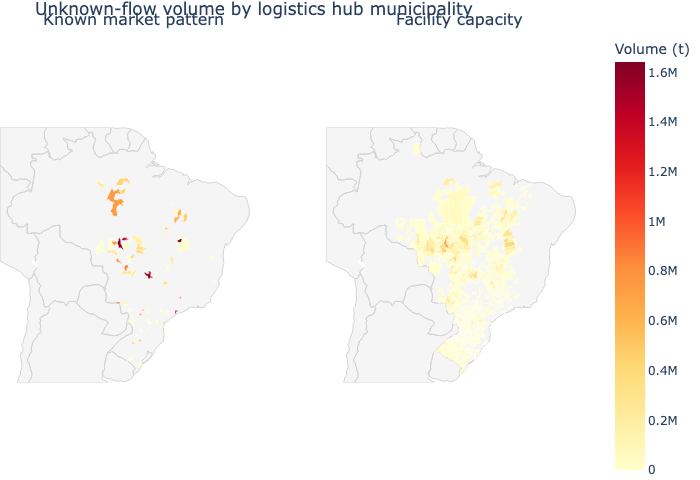
The pattern method concentrates volume in a small number of municipalities with a few very intense hotspots; the facility capacity method spreads the same volume much more broadly across central Brazil.
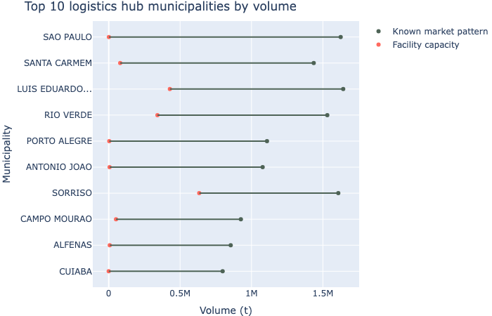
The municipalities that dominate under the pattern method are, almost across the board, barely used by the facility capacity method — confirming that the two methods aren’t just adding a long tail on top of the same core allocation, they disagree about where the bulk of the volume should go.
Production municipality
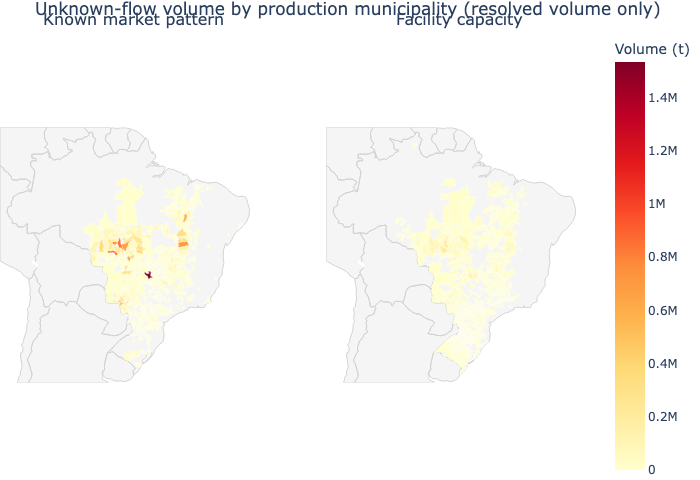
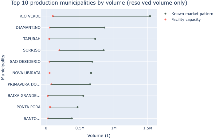
Unlike logistics hub, production municipality is not always resolved — for either method. Where it is resolved, both methods now show comparable municipality-level diversity (see the “production trase id known” query above), so a side-by-side comparison is meaningful, but the two methods resolve very different amounts of volume to begin with:
| Method | Distinct production municipalities | Volume with a production municipality (%) |
|---|---|---|
| Known market pattern | 1,426 | 96.2 |
| Facility capacity | 1,574 | 27.4 |
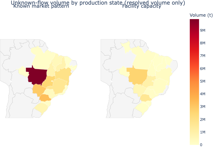
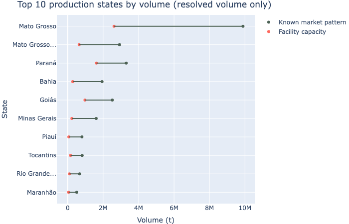
The map and dumbbell below are restricted to the resolved portion of each method’s volume, so they compare like with like — they say nothing about the unresolved share, which the table above already covers.
Analysis 2: The same comparison, aggregated to state level
Logistics hub state
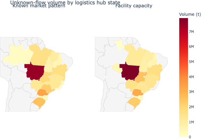
At state level the two methods look far more similar than at municipality level — both are dominated by Mato Grosso, with a similar secondary spread. The divergence between the methods is mostly about which municipality within a state gets the volume, not which state.
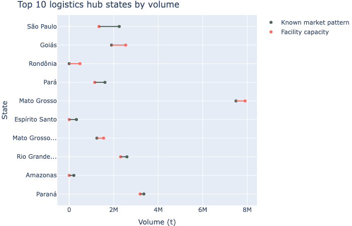
This confirms the map: state by state, the two methods land within a similar order of magnitude of each other almost everywhere in the top 10, unlike the municipality-level dumbbell above where the capacity method’s dot sat right at zero for most of the pattern method’s top picks.
Production state
As in Analysis 1, this is restricted to each method’s resolved production volume — see the table above for how much of each method’s volume that is.
Analysis 3: Are the extra municipalities just tiny and inconsequential?
The capacity method uses far more municipalities (see the headline table), but a raw count doesn’t say whether that’s genuine spread or a long tail of near-empty additions. The inverse Simpson index — the “effective number of categories” implied by a distribution, $1 / \sum_i share_i^2$ — answers that more precisely: it only rises when volume is actually spread more evenly, not just when more near-empty categories are added.
Note the counts below are lower than in the headline table (127 / 1,481)
— this table, like the rest of this section, is filtered to just the
2.4 DISTRIBUTION OF UNKNOWNS branch, whereas the headline table counts
distinct logistics hub municipalities across the whole export file,
including hubs assigned via branches 1–4.1.1 that never went through
unknown-flow allocation.
| Method | Distinct logistics hub municipalities | Inverse Simpson index | As % of raw count | Municipalities \< 0.01% share | Volume held by those tiny municipalities (%) |
|---|---|---|---|---|---|
| Known market pattern | 97 | 30.3 | 31.2 | 19 | 0.07 |
| Facility capacity | 1,460 | 193.4 | 13.2 | 565 | 2.22 |
So: mostly yes, but not entirely. The capacity method’s inverse Simpson index is only about 6-7x the pattern method’s, despite using ~15x as many municipalities — most of that extra count is indeed a long tail of small additions. But “municipalities \< 0.01% share” individually contribute less than 0.01% of the method’s total volume each; the last column sums up their volume together — a couple of percent combined for the capacity method, i.e. what you’d lose if you deleted every single one of them. So: a small but non-trivial amount that a raw “distinct municipalities” count would make look far more dramatic than it is.
Analysis 4: Does the capacity method introduce tiny flows?
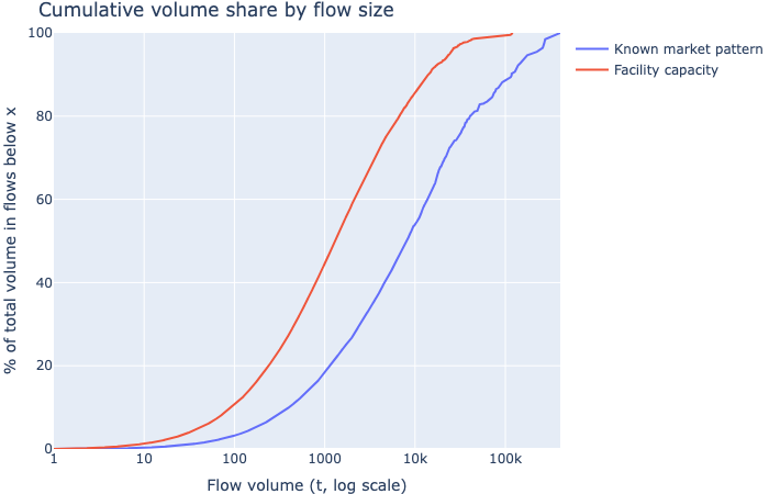
The facility capacity curve sits consistently above and to the left of the pattern method’s, at every cutoff. That means: at any given flow-size threshold, a larger share of the capacity method’s volume is made up of flows smaller than that threshold. So yes — the capacity method does introduce more small flows, not just more municipalities; the two effects go together.
Analysis 5: Histogram overlap between the two methods, across dimensions
Following the “agreement” approach from
comparison_to_secex_exports.qmd
— the share of normalised volume that both sides allocate to the same
bucket, i.e. distributional overlap / histogram intersection,
$\sum_i \min(p_i, q_i)$ — we compare how the two methods split the
shared unknown-origin volume pool, across four increasingly granular
sets of dimensions. branch is normalised first, as in the sanity check
above, since it differs cosmetically by method.
| Dimensions | Buckets | Agreement (%) |
|---|---|---|
| Trade data only (reference — no branch, no geography) | 334 | 99.494 |
| All columns | 248,892 | 0.014 |
| logistics_hub_trase_id | 1,469 | 17.714 |
| production_trase_id | 2,221 | 21.503 |
| production_trase_id + logistics_hub_trase_id | 4,734 | 6.442 |
Are these numbers right? Two checks say yes. First, the assertion
above confirms agreement() returns exactly 100% when comparing a
distribution against itself. Second, the reference row: on trade data
alone — no branch, no geography — agreement is ~99.5%. That’s the real
headline: for a given (exporter, port, country, product, year)
combination, both methods resolve almost exactly the same total volume
into this branch. They agree almost perfectly on how much to allocate;
the four rows below are about where, which is precisely the thing the
two methods are built to disagree on.
Given that, the four requested rows read differently:
logistics_hub_trase_id(17.7%) is a genuinely comparable row — both methods populate this field for (almost) all their volume, so 17.7% is a real measure of how often they pick the same hub. It’s low, consistent with the choropleth and dumbbell above: the two methods concentrate volume in largely different municipalities.production_trase_id(21.5%) is higher, but is a blend of two different effects. Analysis 1 showed the capacity method still leaves the majority of its volume with no production municipality — a big"UNKNOWN"bucket, worth 72.6% of its volume vs. only 3.8% of the pattern method’s. That single bucket contributes 3.8 percentage points of the 21.5% on its own (min(3.8%, 72.6%)). The remaining ~17.7 points come from genuine overlap on resolved production municipalities — and if you restrict to only the volume both methods resolve to a real municipality and renormalise, agreement jumps to ~42.8%. So where the capacity method does resolve production, it agrees with the pattern method’s choice more often than the two methods agree on logistics hub.production_trase_id + logistics_hub_trase_id(6.4%) andAll columns(~0.01%) are both far lower than either single dimension, as expected — requiring two independent low-overlap dimensions to match simultaneously is stricter than either alone.All columnscollapses almost to zero because at that granularity there are more distinct buckets (248,892) than there are rows across both methods combined (248,916) — so an exact match across every dimension simultaneously is close to combinatorially impossible.
Analysis 6: Why does the facility capacity method leave so much production unresolved?
Analysis 1 found the facility capacity method resolves a production municipality for only ~27% of its branch-2.4 volume, against ~96% for the pattern method. A natural hypothesis: the capacity method sends volume to logistics hub municipalities that are scattered across Brazil, and the supply-shed model — which matches production to a logistics hub only within a state-specific distance cutoff — simply cannot find any production within reach of some of these hubs, since export demand exists at every storage municipality regardless of whether soy is grown nearby.
We test this directly against the datasets the supply-shed model
(trase/models/brazil/soy_supply_sheds) itself uses: the farm→silo
cost/distance matrix, the state-specific distance cutoffs, and the
production dataset — reading the same S3 keys as
soy_supply_sheds/preparation.py and replicating the exact cutoff logic
from soy_supply_sheds/model.py (cutoff keyed to the production
municipality’s own state, not the hub’s).
1 of 1,469 logistics hub municipalities (used in branch 2.4 by either method) have no production municipality within their state-specific distance cutoff.
That’s a strong result, but the wrong sign for the hypothesis as stated: almost every hub is technically reachable from some production. So a hub being entirely out of range isn’t the main story. A softer version of the same idea might still hold, though: even a “reachable” hub could have so little production nearby, relative to its demand, that the model can’t fully supply it. We test that too, using the capacity method’s actual per-hub unresolved-production share:
| Production within cutoff, vs. hub demand | Hubs | Total volume (t) | Unresolved production (%) |
|---|---|---|---|
| > 100x (abundant) | 1,443 | 23,383,009 | 71.8 |
| 10-100x | 15 | 2,741,848 | 77.4 |
| 1-10x | 2 | 252,842 | 89.7 |
Even hubs with production reserves hundreds of times their own demand within the cutoff still have a high unresolved-production rate — barely different from scarcer hubs. So neither reachability nor local production abundance explains the gap. The hypothesis, as stated, doesn’t hold up.
Where “UNKNOWN” actually enters the pipeline
If it isn’t geography, the next place to look is the pipeline itself.
Production, silo and crushing geography reach the final export in two
stages: first the supply-shed LP (soy_supply_sheds) solves for
production↔hub assignment and writes solution_exports_*.csv; then
reconcile_supplyshed_and_supplychain (in
soy_2023_2024_v27/post_processing.py) stitches that solution back onto
individual flow rows. Each stage can independently leave volume
unresolved — so we check them separately, using each method’s own raw
supply-shed solution (backed up alongside the final export by
ab_test_s3.py):
| Method | Supply-shed LP solution volume (t) | Unresolved within the LP solution itself (%) |
|---|---|---|
| Known market pattern | 26,863,788 | 3.8 |
| Facility capacity | 26,863,788 | 16.2 |
Both methods’ supply-shed solutions cover the same total volume (confirming the LP fully solves the same demand either way), but the capacity method’s own solution is already ~4x more unresolved than the pattern method’s (consistent with it spanning far more, more thinly-supplied hubs — some real geographic effect after all, just not the binary “out of range” version). Still, at 16% this is nowhere near the ~73% we saw in the final export. Most of the gap opens up after the LP, in the reconciliation stitch:
Of 9,188 distinct (logistics hub, export port) combinations in the final flows, 18,967,421 tonnes — out of 26,377,698 tonnes total — sit in a combination where the supply-shed solution’s known-production volume falls short of what the flows data needs at that exact (hub, port) pairing.
That shortfall alone accounts for almost all of the remaining gap
between the LP’s own 16% and the final export’s 73%.
reconcile_supplyshed_and_supplychain matches on (branch, product,
port, logistics hub) — a finer key than the LP itself uses — and caps
matched volume at min(flows demand, supply-shed supply) for each
combination (stitch_dataframes,
trase/tools/sei_pcs/pandas_utilities.py). The supply-shed LP resolves
production at the hub level; the facility capacity method’s flows are
fragmented across roughly twice as many distinct (hub, port)
combinations as the pattern method produces from the same volume. So
even where a hub has ample production access in aggregate, its LP
solution isn’t broken down finely enough by export port to cover every
combination the flows actually need — and the excess falls through as
unresolved.
Verdict on the hypothesis: not quite as stated, but a related mechanism is real. Logistics hubs being entirely out of reach of production isn’t the driver — reachability is nearly universal, and production abundance within cutoff barely correlates with the unresolved rate. Distance does still matter, but indirectly and more mildly: it makes the supply-shed LP’s own resolution somewhat worse for the capacity method (16% vs 4%). The dominant effect is downstream of the LP entirely — a granularity mismatch in the reconciliation stitch, itself a consequence of the facility capacity method spreading demand across far more (hub, port) combinations than the supply-shed solution was ever resolved at.