View or edit on GitHub

This page is synchronized from trase/data/brazil/soy/indicators/out/q3_2026/qa/comparing_to_previous_results.md. Last modified on 2026-09-20 13:50 CEST by Nicolas Martin. Please view or edit the original file there; changes should be reflected here after a midnight build (CET time), or manually triggering it with a GitHub action (link).

QA Comparison: New vs. Legacy Soy Deforestation & Emissions Indicators

Florian Gollnow 2026-08-30

Setup & Libraries

library(tidyverse)
library(aws.signature)
library(aws.s3)
library(arrow)
library(scales)

aws.signature::use_credentials()

# Helper for text cleaning
str_trans <- function(x) {
  x %>%
    stringi::stri_trans_toupper() %>%
    stringi::stri_trans_general("Latin-ASCII")
}

Data Ingestion & Harmonization

# 1. Load Biome Spatial Mapping Lookup
biomes_lookup <- s3read_using(
  FUN = read_delim,
  delim = ";",
  object = "brazil/spatial/boundaries/ibge/br_municipality_biome/Bioma_Predominante_por_Municipio_2024.csv",
  opts = c("check_region" = TRUE),
  bucket = "trase-storage"
) %>%
  mutate(
    BIOME = str_trans(`Bioma predominante`),
    TRASE_ID = paste0("BR-", `Geocódigo`)
  ) %>%
  select(TRASE_ID, BIOME)

# 2. Load Processed Datasets from S3
df_new <- s3read_using(
  FUN = read_parquet,
  object = "brazil/soy/indicators/out/q3_2026/soy_deforestation_emission_norm_2014_2024_q3_2026_multilevel.parquet",
  opts = c("check_region" = TRUE),
  bucket = "trase-storage"
)

df_legacy <- s3read_using(
  FUN = read_parquet,
  object = "brazil/soy/indicators/out/q4_2025/soy_def_2014_2024_glad_mb_orig_ngb_multilevel_fix_q3_2026.parquet",
  opts = c("check_region" = TRUE),
  bucket = "trase-storage"
)

# 3. Harmonize, Join Metrics & Attach Biome Information
qa_joined <- df_new %>%
  select(
    TRASE_ID,
    YEAR,
    level,
    new_area_ha = SOY_GLAD_HA,
    new_total_def_ha = SOY_DEFORESTATION_5_YEAR_TOTAL,
    new_forest_def_ha = SOY_FOREST_DEFORESTATION_5_YEAR_TOTAL,
    new_non_forest_def_ha = SOY_NON_FOREST_DEFORESTATION_5_YEAR_TOTAL,
    new_total_def_ton = SOY_DEFORESTATION_5_YEAR_TOTAL_NORM_PER_TON,
    new_gross_emiss = CO2_GROSS_EMISSIONS_SOY_DEFORESTATION_5_YEAR_TOTAL,
    new_gross_emiss_forest = CO2_GROSS_EMISSIONS_SOY_FOREST_DEFORESTATION_5_YEAR_TOTAL,
    new_gross_emiss_non_forest = CO2_GROSS_EMISSIONS_SOY_NON_FOREST_DEFORESTATION_5_YEAR_TOTAL,
    new_net_emiss = CO2_NET_EMISSIONS_SOY_DEFORESTATION_5_YEAR_TOTAL
  ) %>%
  inner_join(
    df_legacy %>%
      select(
        TRASE_ID,
        YEAR,
        level,
        leg_area_ha = SOY_GLAD_HA,
        leg_def_ha = SOY_DEFORESTATION_5_YEAR_TOTAL,
        leg_def_ton = SOY_DEFORESTATION_PER_TN_5_YEAR_TOTAL,
        leg_gross_emiss = CO2_GROSS_EMISSIONS_SOY_DEFORESTATION_5_YEAR_TOTAL,
        leg_net_emiss = CO2_NET_EMISSIONS_SOY_DEFORESTATION_5_YEAR_TOTAL
      ),
    by = c("TRASE_ID", "YEAR", "level")
  ) %>%
  left_join(biomes_lookup, by = "TRASE_ID")

Statistical Summaries & Outlier Detection

# 4a. Statistical Summary Table by Spatial Level (Deforestation, Gross & Net Emissions)
qa_summary_by_level <- qa_joined %>%
  group_by(level) %>%
  summarise(
    n_records = n(),
    total_ha_new = sum(new_total_def_ha, na.rm = TRUE),
    total_ha_legacy = sum(leg_def_ha, na.rm = TRUE),
    ha_diff_pct = (total_ha_new - total_ha_legacy) / total_ha_legacy * 100,
    pearson_r_def_ha = cor(new_total_def_ha, leg_def_ha, use = "complete.obs"),
    spearman_r_def_ha = cor(
      new_total_def_ha,
      leg_def_ha,
      method = "spearman",
      use = "complete.obs"
    ),
    mae_def_ha = mean(abs(new_total_def_ha - leg_def_ha), na.rm = TRUE),
    rmse_def_ha = sqrt(mean((new_total_def_ha - leg_def_ha)^2, na.rm = TRUE)),
    pearson_r_intensity = cor(
      new_total_def_ton,
      leg_def_ton,
      use = "complete.obs"
    ),
    total_gross_emiss_new = sum(new_gross_emiss, na.rm = TRUE),
    total_gross_emiss_legacy = sum(leg_gross_emiss, na.rm = TRUE),
    gross_emiss_diff_pct = (total_gross_emiss_new - total_gross_emiss_legacy) /
      total_gross_emiss_legacy *
      100,
    pearson_r_gross_emiss = cor(
      new_gross_emiss,
      leg_gross_emiss,
      use = "complete.obs"
    ),
    spearman_r_gross_emiss = cor(
      new_gross_emiss,
      leg_gross_emiss,
      method = "spearman",
      use = "complete.obs"
    ),
    total_net_emiss_new = sum(new_net_emiss, na.rm = TRUE),
    total_net_emiss_legacy = sum(leg_net_emiss, na.rm = TRUE),
    net_emiss_diff_pct = (total_net_emiss_new - total_net_emiss_legacy) /
      total_net_emiss_legacy *
      100,
    pearson_r_net_emiss = cor(
      new_net_emiss,
      leg_net_emiss,
      use = "complete.obs"
    ),
    spearman_r_net_emiss = cor(
      new_net_emiss,
      leg_net_emiss,
      method = "spearman",
      use = "complete.obs"
    ),
    .groups = "drop"
  )

knitr::kable(
  qa_summary_by_level,
  caption = "QA Statistical Summary by Level of Total Soy Deforestation, Gross & Net Emissions"
)

level	n_records	total_ha_new	total_ha_legacy	ha_diff_pct	pearson_r_def_ha	spearman_r_def_ha	mae_def_ha	rmse_def_ha	pearson_r_intensity	total_gross_emiss_new	total_gross_emiss_legacy	gross_emiss_diff_pct	pearson_r_gross_emiss	spearman_r_gross_emiss	total_net_emiss_new	total_net_emiss_legacy	net_emiss_diff_pct	pearson_r_net_emiss	spearman_r_net_emiss
biome	66	8148210	8285461	-1.656535	0.9972228	0.9967018	5057.20116	10711.7830	0.5828598	1209692883	1236383729	-2.158783	0.9973523	0.9952406	1058473493	780553861	35.60544	0.9857116	0.9876422
country	11	8148210	8285461	-1.656535	0.9949966	0.9818182	16397.57184	19553.5250	0.8333919	1209692883	1236383729	-2.158783	0.9976885	0.9727273	1058473493	780553861	35.60544	0.9955737	0.9636364
municipality	61270	8148210	8285461	-1.656535	0.9915232	0.9542717	8.53944	116.8526	0.3363595	1209692883	1236383729	-2.158783	0.9876614	0.9523298	1058473493	780553861	35.60544	0.9732006	0.9362775
state	297	8148210	8285461	-1.656535	0.9962545	0.9970471	1308.14205	5625.1569	NaN	1209692883	1236383729	-2.158783	0.9938497	0.9962818	1058473493	780553861	35.60544	0.9828536	0.9931134

QA Statistical Summary by Level of Total Soy Deforestation, Gross & Net Emissions

# 4b. Statistical Summary Table by Year (Municipal Level)
qa_summary_by_year <- qa_joined %>%
  filter(level == "municipality") %>%
  group_by(YEAR) %>%
  summarise(
    n_records = n(),
    total_ha_new = sum(new_total_def_ha, na.rm = TRUE),
    total_ha_legacy = sum(leg_def_ha, na.rm = TRUE),
    ha_diff_pct = (total_ha_new - total_ha_legacy) / total_ha_legacy * 100,
    pearson_r_def_ha = cor(new_total_def_ha, leg_def_ha, use = "complete.obs"),
    total_gross_emiss_new = sum(new_gross_emiss, na.rm = TRUE),
    total_gross_emiss_legacy = sum(leg_gross_emiss, na.rm = TRUE),
    gross_emiss_diff_pct = (total_gross_emiss_new - total_gross_emiss_legacy) /
      total_gross_emiss_legacy *
      100,
    pearson_r_gross_emiss = cor(
      new_gross_emiss,
      leg_gross_emiss,
      use = "complete.obs"
    ),
    total_net_emiss_new = sum(new_net_emiss, na.rm = TRUE),
    total_net_emiss_legacy = sum(leg_net_emiss, na.rm = TRUE),
    net_emiss_diff_pct = (total_net_emiss_new - total_net_emiss_legacy) /
      total_net_emiss_legacy *
      100,
    pearson_r_net_emiss = cor(
      new_net_emiss,
      leg_net_emiss,
      use = "complete.obs"
    ),
    .groups = "drop"
  )

knitr::kable(
  qa_summary_by_year,
  caption = "QA Statistical Summary by Year (Total Soy Deforestation, Gross & Net Emissions)"
)

YEAR	n_records	total_ha_new	total_ha_legacy	ha_diff_pct	pearson_r_def_ha	total_gross_emiss_new	total_gross_emiss_legacy	gross_emiss_diff_pct	pearson_r_gross_emiss	total_net_emiss_new	total_net_emiss_legacy	net_emiss_diff_pct	pearson_r_net_emiss
2014	5570	474039.3	466956.0	1.5169261	0.9981936	61209454	61993706	-1.2650515	0.9990232	52536759	37766921	39.10787	0.9826653
2015	5570	701153.4	687934.9	1.9214735	0.9977887	95570730	95660777	-0.0941317	0.9982390	82745459	58892287	40.50305	0.9830934
2016	5570	581025.8	587952.1	-1.1780271	0.9980833	80031590	81661393	-1.9958063	0.9987778	69398164	50848347	36.48067	0.9790400
2017	5570	886167.3	893996.5	-0.8757527	0.9985188	127541983	130613393	-2.3515271	0.9987135	111290592	81291976	36.90231	0.9804314
2018	5570	791910.5	803109.7	-1.3944792	0.9987081	116648628	119573722	-2.4462679	0.9991988	102094497	74695788	36.68039	0.9833212
2019	5570	746709.4	767526.4	-2.7122246	0.9978006	110461606	113980035	-3.0868817	0.9985365	96676280	72053151	34.17356	0.9821933
2020	5570	570702.0	599000.9	-4.7243569	0.9956317	85003167	88298482	-3.7320185	0.9944273	74353547	56431317	31.75937	0.9850333
2021	5570	801386.5	838821.5	-4.4628010	0.9977377	121481795	127375577	-4.6270898	0.9978412	106493175	81997268	29.87405	0.9842048
2022	5570	834106.5	861552.2	-3.1856109	0.9968879	129295872	133286147	-2.9937655	0.9972328	113664715	84834006	33.98485	0.9838024
2023	5570	944922.8	963784.1	-1.9569947	0.9835769	154636229	157180265	-1.6185469	0.9776249	136799054	101475288	34.81021	0.9671373
2024	5570	816086.0	814827.1	0.1545082	0.9658272	127811828	126760232	0.8295951	0.9481672	112421251	80267510	40.05823	0.9357898

QA Statistical Summary by Year (Total Soy Deforestation, Gross & Net Emissions)

# 5a. Outlier & Mismatch Flagging (Top 10 Municipal Total Soy Deforestation Discrepancies)
muni_discrepancies_ha <- qa_joined %>%
  filter(level == "municipality") %>%
  mutate(
    abs_diff_ha = abs(new_total_def_ha - leg_def_ha),
    rel_diff_pct = if_else(
      leg_def_ha > 0,
      (new_total_def_ha - leg_def_ha) / leg_def_ha * 100,
      NA_real_
    )
  ) %>%
  arrange(desc(abs_diff_ha)) %>%
  slice_head(n = 10)

knitr::kable(
  muni_discrepancies_ha %>%
    select(
      TRASE_ID,
      BIOME,
      YEAR,
      new_total_def_ha,
      leg_def_ha,
      abs_diff_ha,
      rel_diff_pct
    ),
  caption = "Top 10 Municipal Total Soy Deforestation Discrepancies (ha)"
)

TRASE_ID	BIOME	YEAR	new_total_def_ha	leg_def_ha	abs_diff_ha	rel_diff_pct
BR-1400100	AMAZONIA	2024	16840.281	2519.173	14321.108	568.48448
BR-1400100	AMAZONIA	2023	17948.633	7351.431	10597.202	144.15156
BR-1400050	AMAZONIA	2024	12533.554	2533.216	10000.338	394.76844
BR-1400159	AMAZONIA	2024	11687.608	1889.453	9798.155	518.57084
BR-1400050	AMAZONIA	2023	11245.050	4412.313	6832.738	154.85615
BR-1400159	AMAZONIA	2023	9966.577	4350.830	5615.747	129.07301
BR-4318309	PAMPA	2023	16789.237	20030.610	3241.373	-16.18210
BR-1400100	AMAZONIA	2022	10134.910	7163.723	2971.187	41.47546
BR-4306601	PAMPA	2022	13771.218	15798.960	2027.742	-12.83465
BR-4306601	PAMPA	2023	13719.616	15687.987	1968.371	-12.54699

Top 10 Municipal Total Soy Deforestation Discrepancies (ha)

# 5b. Outlier & Mismatch Flagging (Top 10 Municipal Gross Emissions Discrepancies)
muni_discrepancies_gross <- qa_joined %>%
  filter(level == "municipality") %>%
  mutate(
    abs_diff_gross = abs(new_gross_emiss - leg_gross_emiss),
    rel_diff_pct = if_else(
      leg_gross_emiss > 0,
      (new_gross_emiss - leg_gross_emiss) / leg_gross_emiss * 100,
      NA_real_
    )
  ) %>%
  arrange(desc(abs_diff_gross)) %>%
  slice_head(n = 10)

knitr::kable(
  muni_discrepancies_gross %>%
    select(
      TRASE_ID,
      BIOME,
      YEAR,
      new_gross_emiss,
      leg_gross_emiss,
      abs_diff_gross,
      rel_diff_pct
    ),
  caption = "Top 10 Municipal Soy Gross CO2 Emissions Discrepancies (tCO2)"
)

TRASE_ID	BIOME	YEAR	new_gross_emiss	leg_gross_emiss	abs_diff_gross	rel_diff_pct
BR-1400100	AMAZONIA	2024	3749424	621753.6	3127670.6	503.04024
BR-1400100	AMAZONIA	2023	4223235	1886194.2	2337041.2	123.90247
BR-1400050	AMAZONIA	2024	2453394	576623.8	1876769.9	325.47559
BR-1400050	AMAZONIA	2023	2464652	1137505.5	1327147.0	116.67170
BR-1400159	AMAZONIA	2024	1543931	258416.3	1285514.3	497.45862
BR-1400159	AMAZONIA	2023	1391829	643311.2	748518.1	116.35396
BR-1400100	AMAZONIA	2022	2355373	1825872.2	529500.3	28.99986
BR-1400100	AMAZONIA	2020	1700664	1265710.7	434953.1	34.36434
BR-1400050	AMAZONIA	2020	1607444	1191162.7	416281.6	34.94750
BR-4306908	PAMPA	2021	1735996	2133056.7	397060.4	-18.61462

Top 10 Municipal Soy Gross CO2 Emissions Discrepancies (tCO2)

# 5c. Outlier & Mismatch Flagging (Top 10 Municipal Net Emissions Discrepancies)
muni_discrepancies_net <- qa_joined %>%
  filter(level == "municipality") %>%
  mutate(
    abs_diff_net = abs(new_net_emiss - leg_net_emiss),
    rel_diff_pct = if_else(
      leg_net_emiss > 0,
      (new_net_emiss - leg_net_emiss) / leg_net_emiss * 100,
      NA_real_
    )
  ) %>%
  arrange(desc(abs_diff_net)) %>%
  slice_head(n = 10)

knitr::kable(
  muni_discrepancies_net %>%
    select(
      TRASE_ID,
      BIOME,
      YEAR,
      new_net_emiss,
      leg_net_emiss,
      abs_diff_net,
      rel_diff_pct
    ),
  caption = "Top 10 Municipal Soy Net CO2 Emissions Discrepancies (tCO2)"
)

TRASE_ID	BIOME	YEAR	new_net_emiss	leg_net_emiss	abs_diff_net	rel_diff_pct
BR-1400100	AMAZONIA	2024	3375761	468709.1	2907052	620.22512
BR-1400100	AMAZONIA	2023	3824247	1435459.2	2388788	166.41277
BR-1400050	AMAZONIA	2024	2175319	423155.0	1752164	414.07131
BR-2911105	CERRADO	2024	4083493	2391635.4	1691858	70.74062
BR-2911105	CERRADO	2023	3596049	2059438.6	1536611	74.61309
BR-2201150	CERRADO	2017	4053387	2537524.9	1515863	59.73784
BR-2101400	CERRADO	2024	3337654	1847990.5	1489663	80.60989
BR-2911105	CERRADO	2017	3548738	2153619.0	1395119	64.78022
BR-1400050	AMAZONIA	2023	2214448	857551.5	1356897	158.22917
BR-2101400	CERRADO	2023	2858833	1519610.3	1339223	88.12936

Top 10 Municipal Soy Net CO2 Emissions Discrepancies (tCO2)

Diagnostic Visualizations: Total Soy Deforestation Area

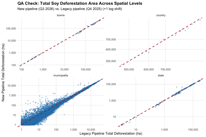
# 6a. Multi-Level Comparison Faceted by Aggregation Level (Total Deforestation)
ggplot(qa_joined, aes(x = leg_def_ha + 1, y = new_total_def_ha + 1)) +
  geom_point(alpha = 0.3, color = "#2c7fb8", size = 1.2) +
  geom_abline(
    intercept = 0,
    slope = 1,
    linetype = "dashed",
    color = "firebrick",
    linewidth = 0.8
  ) +
  scale_x_log10(labels = label_comma()) +
  scale_y_log10(labels = label_comma()) +
  facet_wrap(~level, scales = "free") +
  labs(
    title = "QA Check: Total Soy Deforestation Area Across Spatial Levels",
    subtitle = "New pipeline (Q3 2026) vs. Legacy pipeline (Q4 2025) (+1 log shift)",
    x = "Legacy Pipeline Total Deforestation (ha)",
    y = "New Pipeline Total Deforestation (ha)"
  ) +
  theme_minimal(base_size = 11) +
  theme(
    panel.grid.minor = element_blank(),
    plot.title = element_text(face = "bold")
  )

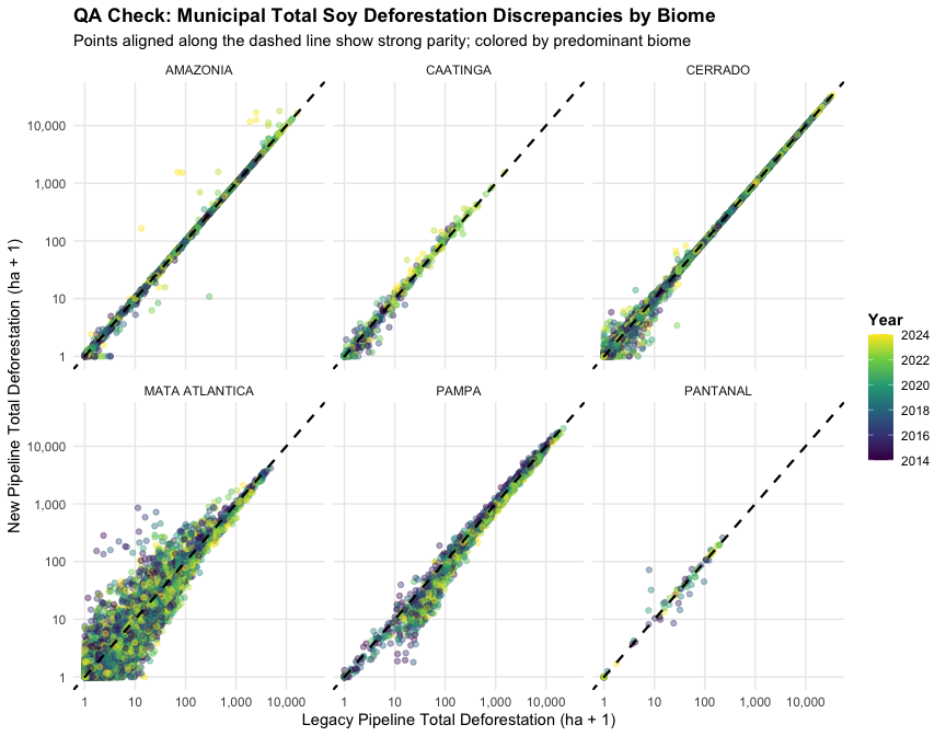
# 6b. Municipal Level Comparison Highlighted and Color-Coded by Biome (Total Deforestation)
qa_muni <- qa_joined %>% filter(level == "municipality", !is.na(BIOME))

ggplot(
  qa_muni,
  aes(x = leg_def_ha + 1, y = new_total_def_ha + 1, color = YEAR)
) +
  geom_point(alpha = 0.4, size = 1.5) +
  geom_abline(
    intercept = 0,
    slope = 1,
    linetype = "dashed",
    color = "black",
    linewidth = 0.8
  ) +
  scale_x_log10(labels = label_comma()) +
  scale_y_log10(labels = label_comma()) +
  scale_color_viridis_c(option = "viridis", na.value = "grey50") +
  labs(
    title = "QA Check: Municipal Total Soy Deforestation Discrepancies by Biome",
    subtitle = "Points aligned along the dashed line show strong parity; colored by predominant biome",
    x = "Legacy Pipeline Total Deforestation (ha + 1)",
    y = "New Pipeline Total Deforestation (ha + 1)",
    color = "Year"
  ) +
  theme_minimal(base_size = 11) +
  theme(
    panel.grid.minor = element_blank(),
    plot.title = element_text(face = "bold"),
    legend.position = "right",
    legend.title = element_text(face = "bold")
  ) +
  facet_wrap(~BIOME)

Diagnostic Visualizations: Soy Deforestation Intensity (Area per Ton)

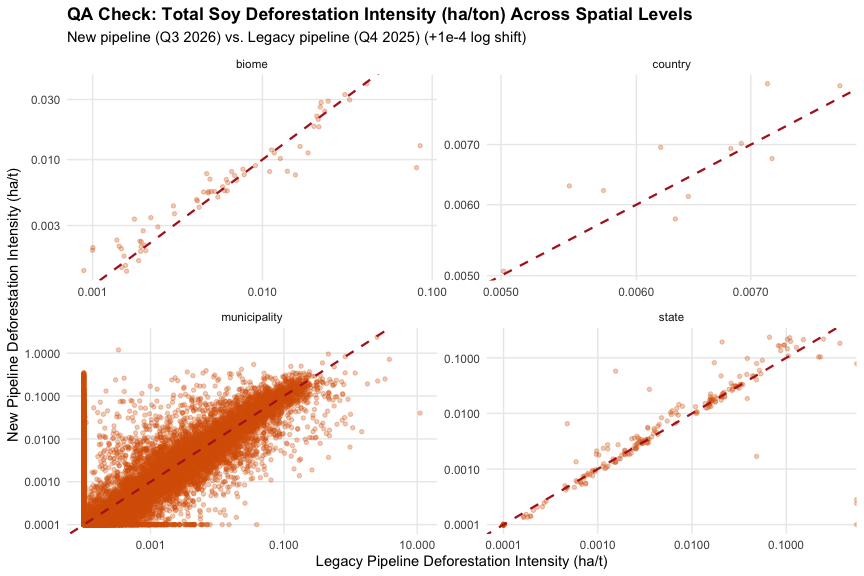
# 7a. Multi-Level Comparison for Intensity Metrics
ggplot(qa_joined, aes(x = leg_def_ton + 1e-4, y = new_total_def_ton + 1e-4)) +
  geom_point(alpha = 0.3, color = "#d95f02", size = 1.2) +
  geom_abline(
    intercept = 0,
    slope = 1,
    linetype = "dashed",
    color = "firebrick",
    linewidth = 0.8
  ) +
  scale_x_log10(labels = label_comma()) +
  scale_y_log10(labels = label_comma()) +
  facet_wrap(~level, scales = "free") +
  labs(
    title = "QA Check: Total Soy Deforestation Intensity (ha/ton) Across Spatial Levels",
    subtitle = "New pipeline (Q3 2026) vs. Legacy pipeline (Q4 2025) (+1e-4 log shift)",
    x = "Legacy Pipeline Deforestation Intensity (ha/t)",
    y = "New Pipeline Deforestation Intensity (ha/t)"
  ) +
  theme_minimal(base_size = 11) +
  theme(
    panel.grid.minor = element_blank(),
    plot.title = element_text(face = "bold")
  )

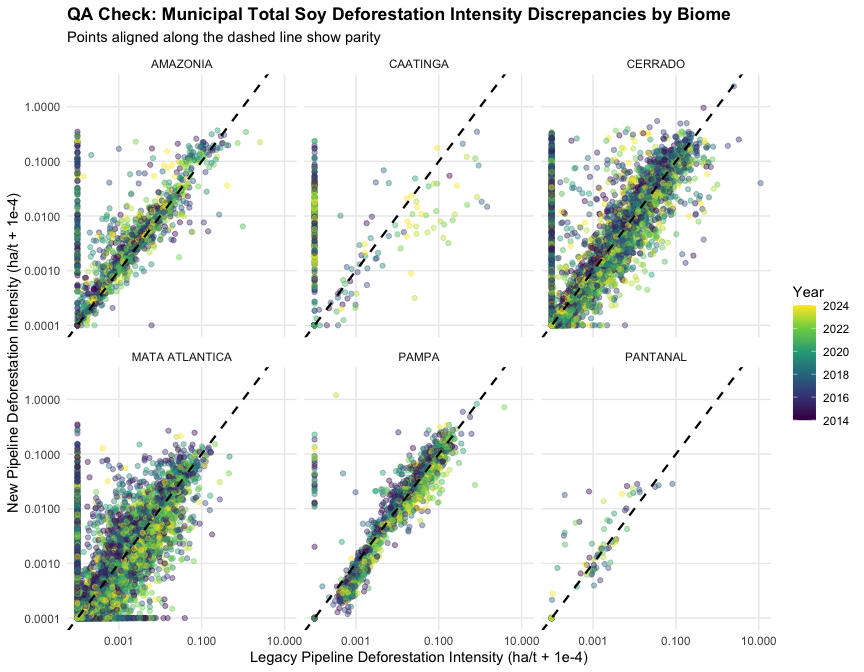
# 7b. Municipal Level Intensity Comparison Highlighted by Biome
ggplot(
  qa_muni,
  aes(x = leg_def_ton + 1e-4, y = new_total_def_ton + 1e-4, color = YEAR)
) +
  geom_point(alpha = 0.4, size = 1.5) +
  geom_abline(
    intercept = 0,
    slope = 1,
    linetype = "dashed",
    color = "black",
    linewidth = 0.8
  ) +
  scale_x_log10(labels = label_comma()) +
  scale_y_log10(labels = label_comma()) +
  scale_color_viridis_c(option = "viridis", na.value = "grey50") +
  labs(
    title = "QA Check: Municipal Total Soy Deforestation Intensity Discrepancies by Biome",
    subtitle = "Points aligned along the dashed line show parity",
    x = "Legacy Pipeline Deforestation Intensity (ha/t + 1e-4)",
    y = "New Pipeline Deforestation Intensity (ha/t + 1e-4)",
    color = "Year"
  ) +
  theme_minimal(base_size = 11) +
  theme(
    panel.grid.minor = element_blank(),
    plot.title = element_text(face = "bold")
  ) +
  facet_wrap(~BIOME)

Diagnostic Visualizations: Gross Emissions

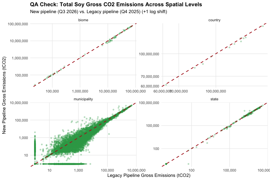
# 8a. Multi-Level Gross Emissions Comparison Faceted by Aggregation Level
ggplot(qa_joined, aes(x = leg_gross_emiss + 1, y = new_gross_emiss + 1)) +
  geom_point(alpha = 0.3, color = "#31a354", size = 1.2) +
  geom_abline(
    intercept = 0,
    slope = 1,
    linetype = "dashed",
    color = "firebrick",
    linewidth = 0.8
  ) +
  scale_x_log10(labels = label_comma()) +
  scale_y_log10(labels = label_comma()) +
  facet_wrap(~level, scales = "free") +
  labs(
    title = "QA Check: Total Soy Gross CO2 Emissions Across Spatial Levels",
    subtitle = "New pipeline (Q3 2026) vs. Legacy pipeline (Q4 2025) (+1 log shift)",
    x = "Legacy Pipeline Gross Emissions (tCO2)",
    y = "New Pipeline Gross Emissions (tCO2)"
  ) +
  theme_minimal(base_size = 11) +
  theme(
    panel.grid.minor = element_blank(),
    plot.title = element_text(face = "bold")
  )

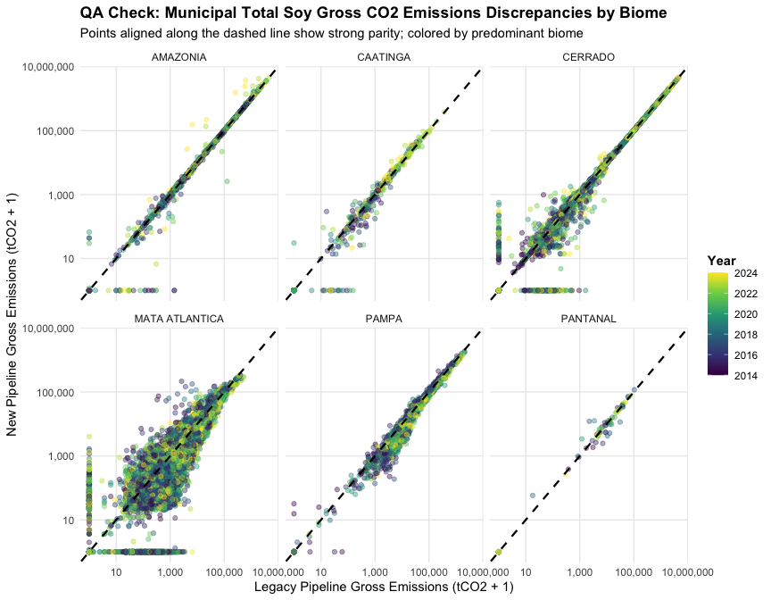
# 8b. Municipal Level Gross Emissions Comparison Highlighted by Biome
ggplot(
  qa_muni,
  aes(x = leg_gross_emiss + 1, y = new_gross_emiss + 1, color = YEAR)
) +
  geom_point(alpha = 0.4, size = 1.5) +
  geom_abline(
    intercept = 0,
    slope = 1,
    linetype = "dashed",
    color = "black",
    linewidth = 0.8
  ) +
  scale_x_log10(labels = label_comma()) +
  scale_y_log10(labels = label_comma()) +
  scale_color_viridis_c(option = "viridis", na.value = "grey50") +
  labs(
    title = "QA Check: Municipal Total Soy Gross CO2 Emissions Discrepancies by Biome",
    subtitle = "Points aligned along the dashed line show strong parity; colored by predominant biome",
    x = "Legacy Pipeline Gross Emissions (tCO2 + 1)",
    y = "New Pipeline Gross Emissions (tCO2 + 1)",
    color = "Year"
  ) +
  theme_minimal(base_size = 11) +
  theme(
    panel.grid.minor = element_blank(),
    plot.title = element_text(face = "bold"),
    legend.position = "right",
    legend.title = element_text(face = "bold")
  ) +
  facet_wrap(~BIOME)

Diagnostic Visualizations: Net Emissions

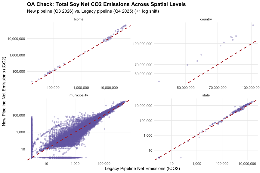
# 9a. Multi-Level Net Emissions Comparison
ggplot(qa_joined, aes(x = leg_net_emiss + 1, y = new_net_emiss + 1)) +
  geom_point(alpha = 0.3, color = "#756bb1", size = 1.2) +
  geom_abline(
    intercept = 0,
    slope = 1,
    linetype = "dashed",
    color = "firebrick",
    linewidth = 0.8
  ) +
  scale_x_log10(labels = label_comma()) +
  scale_y_log10(labels = label_comma()) +
  facet_wrap(~level, scales = "free") +
  labs(
    title = "QA Check: Total Soy Net CO2 Emissions Across Spatial Levels",
    subtitle = "New pipeline (Q3 2026) vs. Legacy pipeline (Q4 2025) (+1 log shift)",
    x = "Legacy Pipeline Net Emissions (tCO2)",
    y = "New Pipeline Net Emissions (tCO2)"
  ) +
  theme_minimal(base_size = 11) +
  theme(
    panel.grid.minor = element_blank(),
    plot.title = element_text(face = "bold")
  )

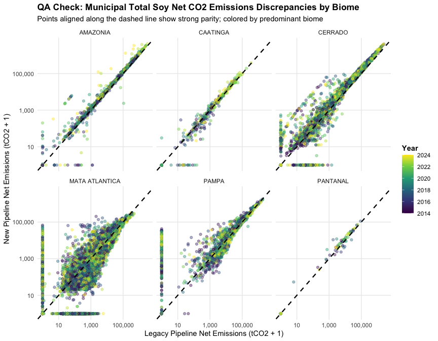
# 9b. Municipal Level Net Emissions Comparison Highlighted by Biome
ggplot(
  qa_muni,
  aes(x = leg_net_emiss + 1, y = new_net_emiss + 1, color = YEAR)
) +
  geom_point(alpha = 0.4, size = 1.5) +
  geom_abline(
    intercept = 0,
    slope = 1,
    linetype = "dashed",
    color = "black",
    linewidth = 0.8
  ) +
  scale_x_log10(labels = label_comma()) +
  scale_y_log10(labels = label_comma()) +
  scale_color_viridis_c(option = "viridis", na.value = "grey50") +
  labs(
    title = "QA Check: Municipal Total Soy Net CO2 Emissions Discrepancies by Biome",
    subtitle = "Points aligned along the dashed line show strong parity; colored by predominant biome",
    x = "Legacy Pipeline Net Emissions (tCO2 + 1)",
    y = "New Pipeline Net Emissions (tCO2 + 1)",
    color = "Year"
  ) +
  theme_minimal(base_size = 11) +
  theme(
    panel.grid.minor = element_blank(),
    plot.title = element_text(face = "bold"),
    legend.position = "right",
    legend.title = element_text(face = "bold")
  ) +
  facet_wrap(~BIOME)

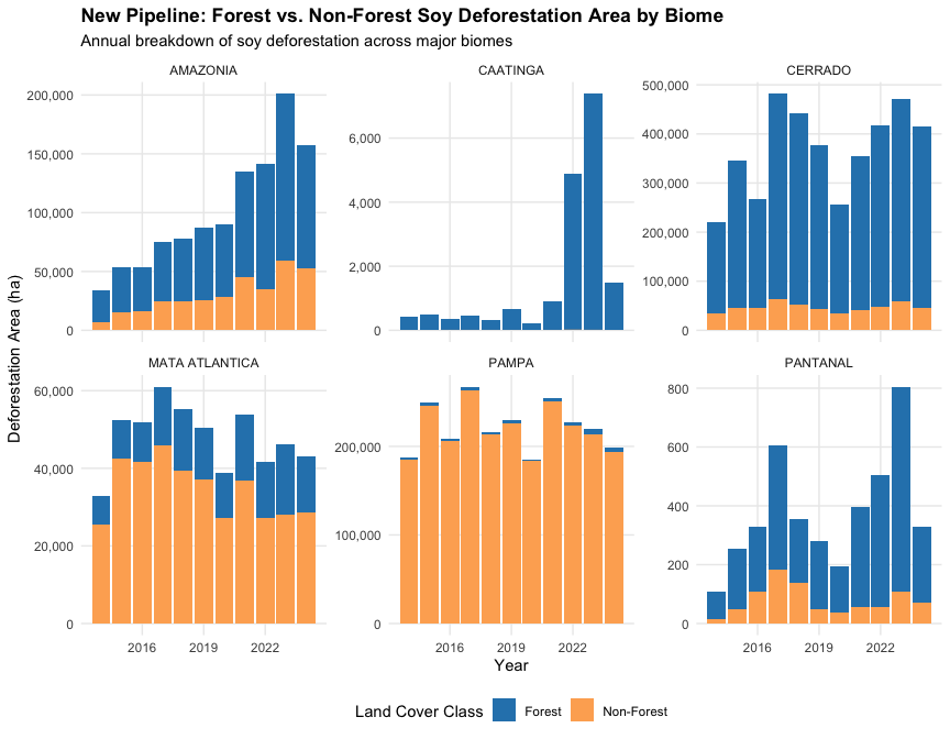
Internal Validation: Forest vs. Non-Forest Breakdown (New Pipeline)

# 10a. Forest vs Non-Forest Soy Deforestation Trends over Time by Biome
df_fn_long_ha <- qa_muni %>%
  group_by(YEAR, BIOME) %>%
  summarise(
    Forest = sum(new_forest_def_ha, na.rm = TRUE),
    `Non-Forest` = sum(new_non_forest_def_ha, na.rm = TRUE),
    .groups = "drop"
  ) %>%
  pivot_longer(
    cols = c(Forest, `Non-Forest`),
    names_to = "land_cover",
    values_to = "deforestation_ha"
  )

ggplot(df_fn_long_ha, aes(x = YEAR, y = deforestation_ha, fill = land_cover)) +
  geom_col(position = "stack") +
  scale_y_continuous(labels = label_comma()) +
  scale_fill_manual(
    values = c("Forest" = "#2b83ba", "Non-Forest" = "#fdae61")
  ) +
  labs(
    title = "New Pipeline: Forest vs. Non-Forest Soy Deforestation Area by Biome",
    subtitle = "Annual breakdown of soy deforestation across major biomes",
    x = "Year",
    y = "Deforestation Area (ha)",
    fill = "Land Cover Class"
  ) +
  theme_minimal(base_size = 11) +
  theme(
    panel.grid.minor = element_blank(),
    plot.title = element_text(face = "bold"),
    legend.position = "bottom"
  ) +
  facet_wrap(~BIOME, scales = "free_y")

# 10b. Forest vs Non-Forest Soy Gross CO2 Emissions Trends over Time by Biome
df_fn_long_emiss <- qa_muni %>%
  group_by(YEAR, BIOME) %>%
  summarise(
    Forest = sum(new_gross_emiss_forest, na.rm = TRUE),
    `Non-Forest` = sum(new_gross_emiss_non_forest, na.rm = TRUE),
    .groups = "drop"
  ) %>%
  pivot_longer(
    cols = c(Forest, `Non-Forest`),
    names_to = "land_cover",
    values_to = "emissions_tco2"
  )

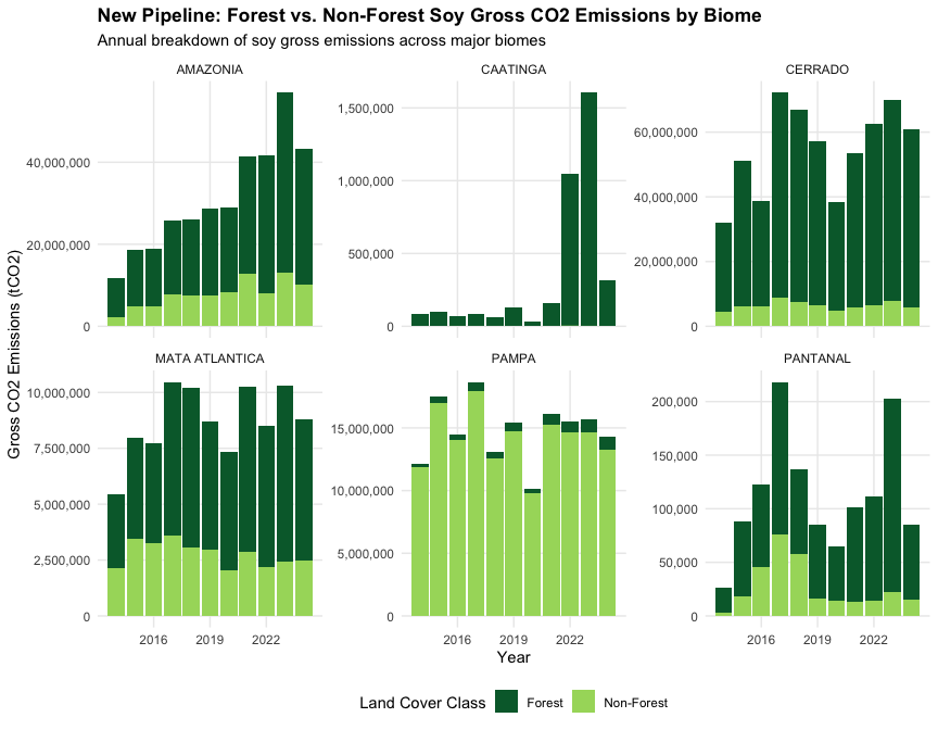
ggplot(df_fn_long_emiss, aes(x = YEAR, y = emissions_tco2, fill = land_cover)) +
  geom_col(position = "stack") +
  scale_y_continuous(labels = label_comma()) +
  scale_fill_manual(
    values = c("Forest" = "#006837", "Non-Forest" = "#a6d96a")
  ) +
  labs(
    title = "New Pipeline: Forest vs. Non-Forest Soy Gross CO2 Emissions by Biome",
    subtitle = "Annual breakdown of soy gross emissions across major biomes",
    x = "Year",
    y = "Gross CO2 Emissions (tCO2)",
    fill = "Land Cover Class"
  ) +
  theme_minimal(base_size = 11) +
  theme(
    panel.grid.minor = element_blank(),
    plot.title = element_text(face = "bold"),
    legend.position = "bottom"
  ) +
  facet_wrap(~BIOME, scales = "free_y")