View or edit on GitHub
This page is synchronized from trase/data/brazil/logistics/silos/silos_map_v3/qa/qa_silos.ipynb. Last modified on 2026-06-21 06:35 CEST by GitHub Actions.
Please view or edit the original file there; changes should be reflected here after a midnight build (CET time),
or manually triggering it with a GitHub action (link).
from trase.tools.aws.aws_helpers import read_geojson
import pandas as pd
import matplotlib.pyplot as plt
import numpy as np
Config Varaibles
PATH_SILOS = 'brazil/logistics/silos/silo_map_v3/silos_consolidated_capacity_brazil_2024_2.geojson'

PATH_STATES = 'brazil/spatial/boundaries/ibge/2023/br_states_wgs84_2023.geojson'

PATH_BIOMES = 'brazil/spatial/boundaries/boundaries_biomes/spatial/old/BRAZIL_BIOMES.geojson'
Input Data
df_states = read_geojson(key=PATH_STATES, bucket='trase-storage')

df_biomes = read_geojson(key=PATH_BIOMES, bucket='trase-storage')

df_silos = read_geojson(key=PATH_SILOS, bucket='trase-storage')

df_silos['year'] = pd.to_numeric(
    df_silos['start_activity_date'].str.split('-').str[0],
    errors='coerce'
).astype('Int64')

df_silos = df_silos.replace({
    'source_metadata': {
        'cnpj': 'Receita Federal',
        'sicarm': 'SICARM',
        'gmaps': 'Google Maps'
    }
})

df_silos.loc[
    (df_silos['source_metadata'] == 'Google Maps') &
    (df_silos['methodology'] == 'EOFM'),
    'source_metadata'
] = 'Google Maps + Gemini'
Count facilities per dataset
import geopandas as gpd

# 1. Garantir que todos os GeoDataFrames estejam no mesmo sistema de coordenadas (CRS)
# Isso é fundamental para que a interseção espacial funcione
df_silos = df_silos.to_crs(df_states.crs)
df_biomes = df_biomes.to_crs(df_states.crs)

# --- Para os Estados ---

# Faz o spatial join: associa cada ponto de silo ao estado correspondente
silos_with_state = gpd.sjoin(df_silos, df_states, how="inner", predicate="within")

# Conta as ocorrências e mapeia para o df_states original
# (Substitua 'id_state' pela coluna que identifica unicamente o estado no seu df_states)
state_counts = silos_with_state.groupby('index_right').size()
df_states['n_silos'] = df_states.index.map(state_counts).fillna(0).astype(int)

# --- Para os Biomas ---

# Faz o spatial join: associa cada ponto de silo ao bioma correspondente
silos_with_biome = gpd.sjoin(df_silos, df_biomes, how="inner", predicate="within")

# Conta as ocorrências e mapeia para o df_biomes original
# (Substitua 'id_biome' pela coluna que identifica unicamente o bioma no seu df_biomes)
biome_counts = silos_with_biome.groupby('index_right').size()
df_biomes['n_silos'] = df_biomes.index.map(biome_counts).fillna(0).astype(int)
QA - Questions
What is the total amount of silos mapped by method?
grouped = (
    df_silos
    .groupby(['methodology'])
    .size()
    .reset_index(name='count')
)

grouped['percentage'] = (
    grouped['count'] /
    grouped['count'].sum()
) * 100

grouped
| methodology | count | percentage | |
|---|---|---|---|
| 0 | DIVERSA | 8253 | 88.022611 |
| 1 | EOFM | 1123 | 11.977389 |
grouped = (
    df_silos
    .groupby(['methodology', 'source_metadata'])
    .size()
    .reset_index(name='count')
)

grouped['percentage'] = (
    grouped['count'] /
    grouped.groupby('methodology')['count'].transform('sum')
) * 100

grouped
| methodology | source_metadata | count | percentage | |
|---|---|---|---|---|
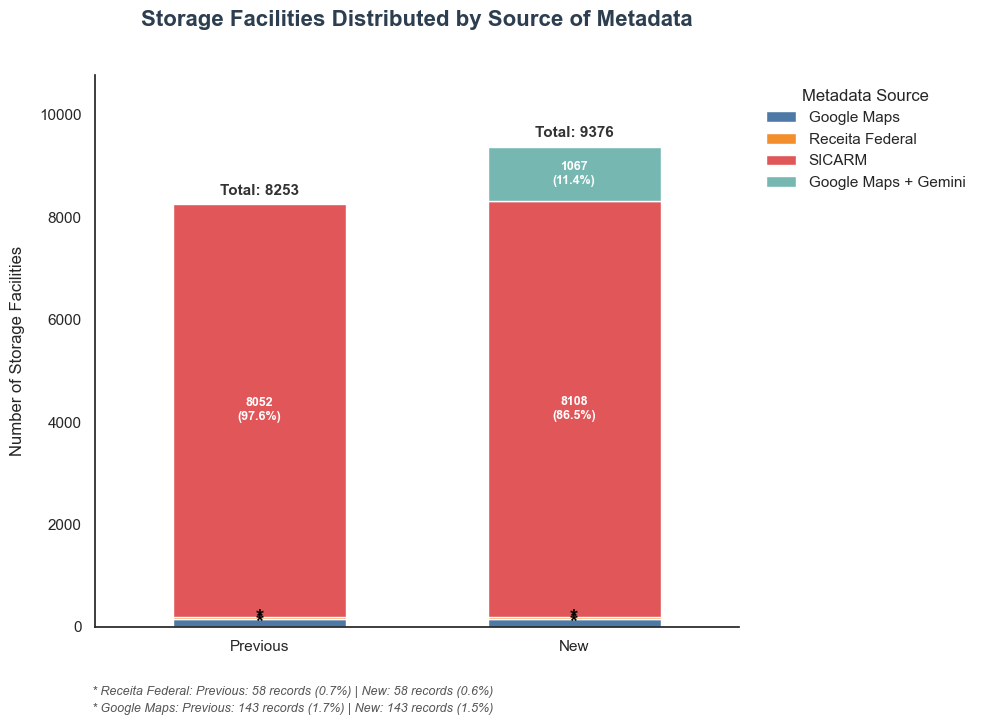
| 0 | DIVERSA | Google Maps | 143 | 1.732703 |
| 1 | DIVERSA | Receita Federal | 58 | 0.702775 |
| 2 | DIVERSA | SICARM | 8052 | 97.564522 |
| 3 | EOFM | Google Maps + Gemini | 1067 | 95.013357 |
| 4 | EOFM | SICARM | 56 | 4.986643 |
How many unique companies?
grouped = (
    df_silos[df_silos['cnpj'].str.len() > 11]
    .groupby(['cnpj'])
    .size()
    .reset_index(name='count')
)

grouped['count'].sum()
5579
How many Tax Numbers were retrived ?
# Filtro base
cnpj_len = df_silos['cnpj'].str.len()
total = len(df_silos)

# Contagens
cnpjs_count = df_silos[cnpj_len == 14]['cnpj'].count()
cpf_count = df_silos[cnpj_len == 11]['cnpj'].count()
# Usamos a lógica de exclusão para pegar o que não é nem CPF nem CNPJ
nulls_count = df_silos[((cnpj_len != 11) & (cnpj_len != 14)) | (df_silos['cnpj'].isna())]['cnpj'].size

# Cálculos de Percentual
pct_cnpj = (cnpjs_count / total) * 100
pct_cpf = (cpf_count / total) * 100
pct_nulls = (nulls_count / total) * 100

print(f"Total de registros: {total}")
print(f"CNPJs: {cnpjs_count} ({pct_cnpj:.2f}%)")
print(f"CPFs:  {cpf_count} ({pct_cpf:.2f}%)")
print(f"Outros/Nulos: {nulls_count} ({pct_nulls:.2f}%)")
Total de registros: 9376
CNPJs: 5579 (59.50%)
CPFs:  3299 (35.19%)
Outros/Nulos: 498 (5.31%)
How many Tax Numbers were retrived using EOFM ?
# Filtro base
is_eofm = df_silos['methodology'] == 'EOFM'
total_eofm = is_eofm.sum() # Total de registros no grupo EOFM
cnpj_len = df_silos['cnpj'].str.len()

# Contagens
cnpjs_by_eofm = df_silos[is_eofm & (cnpj_len == 14)]['cnpj'].count()
cpf_by_eofm = df_silos[is_eofm & (cnpj_len == 11)]['cnpj'].count()

# Lógica de Outros/Nulos para o grupo EOFM
nulls_by_eofm = df_silos[
    is_eofm &
    (
        ((cnpj_len != 11) & (cnpj_len != 14)) |
        (df_silos['cnpj'].isna())
    )
]['cnpj'].size

# Cálculos de Percentual (evitando divisão por zero se o grupo for vazio)
pct_cnpj = (cnpjs_by_eofm / total_eofm * 100) if total_eofm > 0 else 0
pct_cpf  = (cpf_by_eofm / total_eofm * 100) if total_eofm > 0 else 0
pct_null = (nulls_by_eofm / total_eofm * 100) if total_eofm > 0 else 0

print(f"--- Estatísticas EOFM only (Total: {total_eofm}) ---")
print(f"CNPJs: {cnpjs_by_eofm:>5} ({pct_cnpj:>6.2f}%)")
print(f"CPFs:  {cpf_by_eofm:>5} ({pct_cpf:>6.2f}%)")
print(f"Nulos: {nulls_by_eofm:>5} ({pct_null:>6.2f}%)")
--- Estatísticas EOFM only (Total: 1123) ---
CNPJs:   702 ( 62.51%)
CPFs:     38 (  3.38%)
Nulos:   383 ( 34.11%)
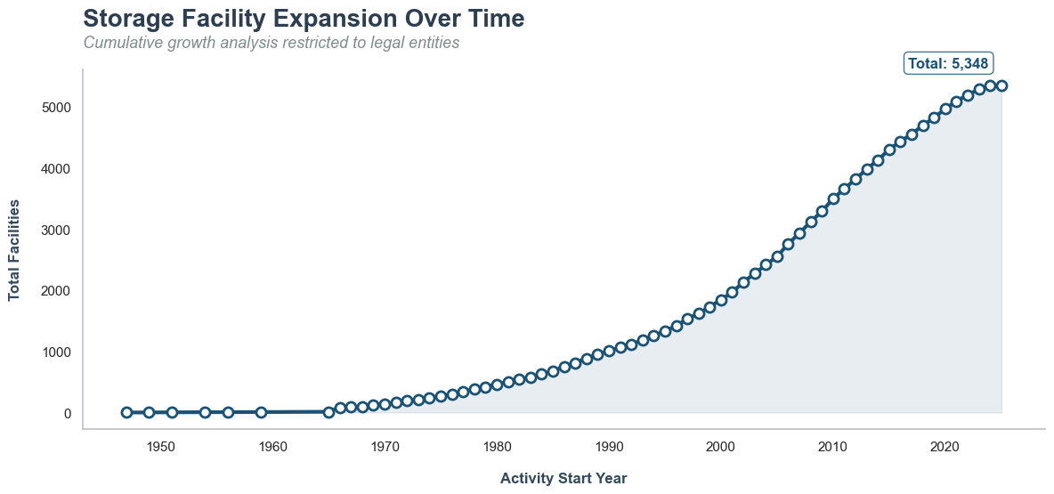
What is the silo expansion for companies?
import matplotlib.pyplot as plt
import seaborn as sns

sns.set_theme(style="white", font="sans-serif")
plt.rcParams['figure.dpi'] = 100


count_per_year = df_silos['year'].value_counts().sort_index()
cumulative_count = count_per_year.cumsum()


fig, ax = plt.subplots(figsize=(12, 7))

# Plotagem
ax.plot(cumulative_count.index, cumulative_count.values,
        color='#1A5276', linewidth=3, marker='o',
        markersize=8, markerfacecolor='white', markeredgewidth=2)

ax.fill_between(cumulative_count.index, cumulative_count.values,
                color='#1A5276', alpha=0.1)


ax.text(0, 1.12, 'Storage Facility Expansion Over Time',
        transform=ax.transAxes, fontsize=20, fontweight='bold', color='#2C3E50')


ax.text(0, 1.06, 'Cumulative growth analysis restricted to legal entities',
        transform=ax.transAxes, fontsize=13, color='#7F8C8D', style='italic')


ax.set_xlabel('Activity Start Year', fontsize=12, fontweight='bold', labelpad=15, color='#34495E')
ax.set_ylabel('Total Facilities', fontsize=12, fontweight='bold', labelpad=15, color='#34495E')


ax.spines['top'].set_visible(False)
ax.spines['right'].set_visible(False)
ax.spines['left'].set_color('#BDC3C7')
ax.spines['bottom'].set_color('#BDC3C7')
ax.grid(False)


last_year = cumulative_count.index[-1]
last_val = cumulative_count.values[-1]

ax.annotate(f'Total: {last_val:,}',
            xy=(last_year, last_val),
            xytext=(-10, 15),
            textcoords='offset points',
            ha='right',
            fontsize=12, fontweight='bold', color='#1A5276',
            bbox=dict(boxstyle='round,pad=0.3', fc='white', ec='#1A5276', alpha=0.8))

footer_text = (
    "*This analysis exclusively covers legal entities. Data regarding natural persons and individual private records\n"
    "are strictly excluded from this management system to ensure privacy and regulatory compliance."
)

# plt.figtext(0.02, 0.05, footer_text,
#             horizontalalignment='left',
#             fontsize=10,
#             color='#95A5A6',
#             style='italic',
#             linespacing=1.2)

plt.tight_layout(rect=[0, 0.08, 1, 0.92])
plt.show()
What is the source metadata distribution ?
# 1. Preparação dos Dados (Tradução e Organização)
previous_silos = df_silos.query('methodology == "DIVERSA"')
new_silos = df_silos.copy()

prev_counts = previous_silos.groupby(['source_metadata']).size().reset_index(name='count')
new_counts = new_silos.groupby(['source_metadata']).size().reset_index(name='count')

df_prev = prev_counts.pivot_table(columns=['source_metadata'], values='count')
df_new = new_counts.pivot_table(columns=['source_metadata'], values='count')

df_prev['version'] = 'Previous'
df_new['version'] = 'New'

df_plot = pd.concat([df_prev, df_new]).set_index('version')
df_plot.rename_axis(None, inplace=True)

# 2. Geração da Nota de Rodapé para Múltiplas Classes (English)
# Mapeamos as classes para símbolos e calculamos os valores
special_sources = {
    'Receita Federal': '*',
    'Google Maps': '*'
}

footer_lines = []
for source, symbol in special_sources.items():
    if source in df_plot.columns:
        details = []
        for version in df_plot.index:
            val = df_plot.loc[version, source]
            total = df_plot.loc[version].sum()
            perc = (val / total) * 100
            details.append(f"{version}: {int(val)} records ({perc:.1f}%)")
        footer_lines.append(f"{symbol} {source}: {' | '.join(details)}")

full_footer_text = "\n".join(footer_lines)

# 3. Configuração do Gráfico
fig, ax = plt.subplots(figsize=(10, 8), dpi=100)
colors = ['#4E79A7', '#F28E2B', '#E15759', '#76B7B2', '#59A14F', '#EDC948']

df_plot.plot(kind='bar', stacked=True, ax=ax, color=colors, width=0.55, edgecolor='white', linewidth=1)

# 4. Anotações Dinâmicas
for i, (idx, row) in enumerate(df_plot.iterrows()):
    total_bar = row.sum()
    cumulative_height = 0

    for col_name, value in row.items():
        if value > 0:
            percentage = (value / total_bar) * 100
            pos_y = cumulative_height + (value / 2)

            # --- Lógica para Notas de Rodapé (Símbolos) ---
            if col_name in special_sources:
                symbol = special_sources[col_name]
                ax.text(i, pos_y, symbol, ha='center', va='center',
                        fontweight='bold', fontsize=15, color='black')

            # --- Segmentos Normais (> 5%) ---
            elif percentage > 5:
                label = f'{int(value)}\n({percentage:.1f}%)'
                ax.text(i, pos_y, label, ha='center', va='center',
                        color='white', fontweight='bold', fontsize=9)

            cumulative_height += value

    # --- Total no Topo ---
    ax.text(i, total_bar + (total_bar * 0.015), f'Total: {int(total_bar)}',
            ha='center', va='bottom', fontweight='extra bold', fontsize=11, color='#333333')

# 5. Estilização (English)
ax.set_title('Storage Facilities Distributed by Source of Metadata', fontsize=16, pad=35, fontweight='bold', color='#2c3e50')
ax.set_ylabel('Number of Storage Facilities', fontsize=12, labelpad=10)
ax.tick_params(axis='x', rotation=0, labelsize=11)

# Ajuste do limite Y para não cortar o total
ax.set_ylim(0, df_plot.sum(axis=1).max() * 1.15)

# Limpeza visual
ax.spines['top'].set_visible(False)
ax.spines['right'].set_visible(False)
ax.legend(title='Metadata Source', bbox_to_anchor=(1.02, 1), loc='upper left', frameon=False)

# 6. Inserção da Nota de Rodapé Multilinha
plt.figtext(0.1, 0.05, full_footer_text, ha='left', fontsize=9,
            fontweight='medium', style='italic', color='#555555',
            linespacing=1.5)

# Ajuste fino do layout para acomodar as duas linhas de rodapé
plt.tight_layout(rect=[0, 0.1, 1, 0.95])
plt.show()
1067+143+58
1268
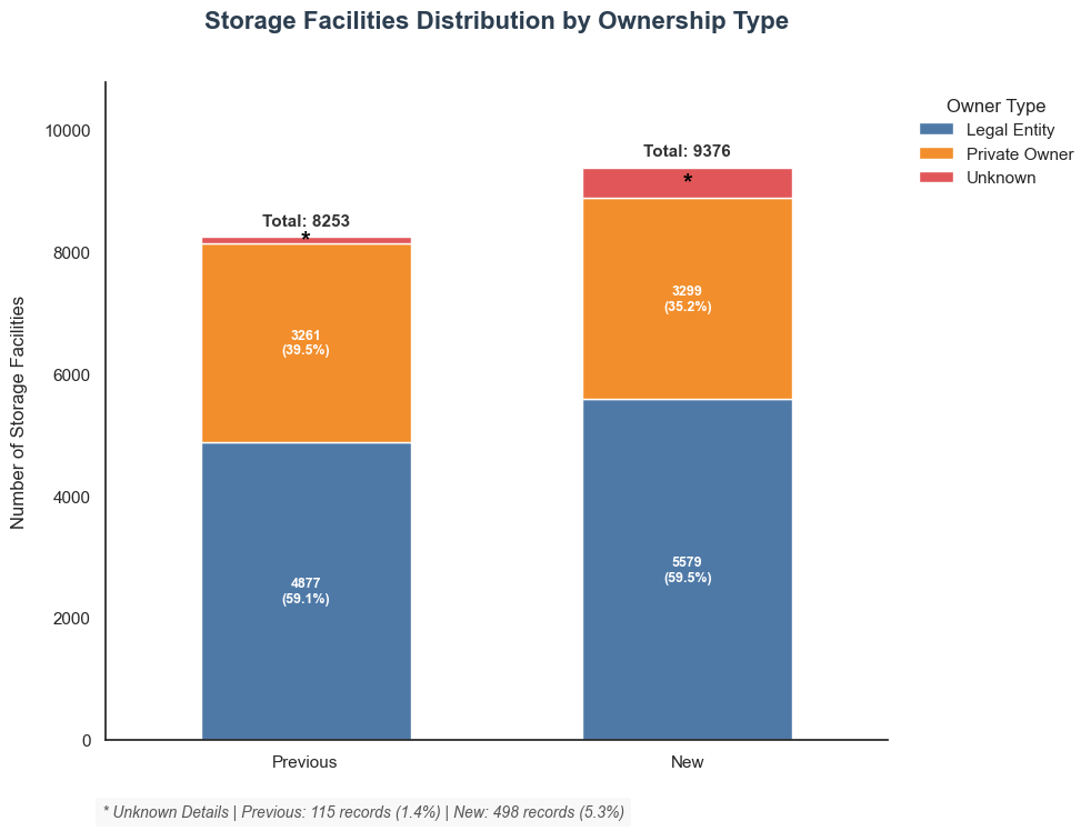
What is the type of facility owner by dataset version?
# 1. Função de Classificação
def classify_owner_type(df, column_name='cnpj'):
    """
    Classifies owners based on the length of the identification string.
    14 digits: Legal Entity | 11 digits: Private Owner | Others: Unknown
    """
    # Limpeza de caracteres não numéricos
    clean_series = df[column_name].astype(str).str.replace(r'\D', '', regex=True)

    conditions = [
        (clean_series.str.len() == 14),
        (clean_series.str.len() == 11)
    ]
    choices = ['Legal Entity', 'Private Owner']

    df['owner_type'] = np.select(conditions, choices, default='Unknown')
    return df

# 2. Aplicação e Preparação dos Dados
new_silos = classify_owner_type(new_silos)
previous_silos = classify_owner_type(previous_silos)

# Contagem e Pivotagem
prev_counts = previous_silos.groupby(['owner_type']).size().reset_index(name='count')
new_counts = new_silos.groupby(['owner_type']).size().reset_index(name='count')

df_prev = prev_counts.pivot_table(columns=['owner_type'], values='count')
df_new = new_counts.pivot_table(columns=['owner_type'], values='count')

df_prev['version'] = 'Previous'
df_new['version'] = 'New'

df_plot = pd.concat([df_prev, df_new]).set_index('version')
df_plot.rename_axis(None, inplace=True)

# 3. Geração da Nota de Rodapé para "Unknown"
special_sources = {'Unknown': '*'}
footer_parts = []

if 'Unknown' in df_plot.columns:
    for version in df_plot.index:
        val = df_plot.loc[version, 'Unknown']
        total = df_plot.loc[version].sum()
        perc = (val / total) * 100
        footer_parts.append(f"{version}: {int(val)} records ({perc:.1f}%)")
    unknown_footer_text = f"* Unknown Details | {' | '.join(footer_parts)}"
else:
    unknown_footer_text = ""

# 4. Configuração do Gráfico
fig, ax = plt.subplots(figsize=(10, 8), dpi=100)
# Paleta: Legal Entity (Azul), Private Owner (Laranja), Unknown (Vermelho/Cinza)
colors = ['#4E79A7', '#F28E2B', '#E15759']

df_plot.plot(kind='bar', stacked=True, ax=ax, color=colors, width=0.55, edgecolor='white', linewidth=1)

# 5. Anotações Dinâmicas
for i, (idx, row) in enumerate(df_plot.iterrows()):
    total_bar = row.sum()
    cumulative_height = 0

    for col_name, value in row.items():
        if value > 0:
            percentage = (value / total_bar) * 100
            pos_y = cumulative_height + (value / 2)

            # --- CASO ESPECIAL: Unknown (Símbolo *) ---
            if col_name == 'Unknown':
                ax.text(i, pos_y, '*', ha='center', va='center',
                        fontweight='bold', fontsize=16, color='black')

            # --- SEGMENTOS NORMAIS (Apenas se > 5%) ---
            elif percentage > 5:
                label = f'{int(value)}\n({percentage:.1f}%)'
                ax.text(i, pos_y, label, ha='center', va='center',
                        color='white', fontweight='bold', fontsize=9)

            cumulative_height += value

    # --- TOTAL NO TOPO ---
    ax.text(i, total_bar + (total_bar * 0.015), f'Total: {int(total_bar)}',
            ha='center', va='bottom', fontweight='extra bold', fontsize=11, color='#333333')

# 6. Estilização (English)
ax.set_title('Storage Facilities Distribution by Ownership Type', fontsize=16, pad=35, fontweight='bold', color='#2c3e50')
ax.set_ylabel('Number of Storage Facilities', fontsize=12, labelpad=10)
ax.tick_params(axis='x', rotation=0, labelsize=11)

# Ajuste do limite Y
ax.set_ylim(0, df_plot.sum(axis=1).max() * 1.15)

# Limpeza visual
ax.spines['top'].set_visible(False)
ax.spines['right'].set_visible(False)
ax.legend(title='Owner Type', bbox_to_anchor=(1.02, 1), loc='upper left', frameon=False)

# Inserção da Nota de Rodapé
if unknown_footer_text:
    plt.figtext(0.1, 0.02, unknown_footer_text, ha='left', fontsize=10,
                fontweight='medium', style='italic', color='#555555',
                bbox=dict(facecolor='grey', alpha=0.05, edgecolor='none'))

plt.tight_layout(rect=[0, 0.05, 1, 0.95])
plt.show()
/Users/jailsonsoares/repos/TRASE/.venv/lib/python3.11/site-packages/geopandas/geodataframe.py:1969: SettingWithCopyWarning:
A value is trying to be set on a copy of a slice from a DataFrame.
Try using .loc[row_indexer,col_indexer] = value instead

See the caveats in the documentation: https://pandas.pydata.org/pandas-docs/stable/user_guide/indexing.html#returning-a-view-versus-a-copy
  super().__setitem__(key, value)
9376-8253
1123
5579-4877
702
Fix CNPJ mannualy
# UPDATE silos_local
# SET
#     cnpj = '44940762000143',
#     cnae = 5211701,
#     cnae_name = 'Armazéns gerais - emissão de warrant'
# WHERE idx = 89;