View or edit on GitHub
This page is synchronized from trase/products/analysis/reports/manuscripts/ZDC_EFFECTIVENESS/CLEAN_BEEF_ZDC_MARKETSHARE.md. Last modified on 2025-12-15 23:00 CET by Trase Admin.
Please view or edit the original file there; changes should be reflected here after a midnight build (CET time),
or manually triggering it with a GitHub action (link).
Calculate ZDC coverage in the BR-cattle sector
Erasmus 2025-05-06
Workflow
- Take the list of slaughterhouses, as provided by Ministry of Agriculture (MAPA) and the Brazilian sanitary inspection system (Sistema Brasileiro de Inspeção de Produtos de Origem Animal, SISBI). This includes most large slaughterhouses in Brazil (i.e. those who have made Zero Deforestation Commitments, ZDCs), but misses uninspected slaughter - as discussed below.
-
Add the slaughterhouse capacities (head/yr) of each facility. The capacities are estimated from animal movement (GTA) data, following the do Pasto ao Prato Cerrado report. Specifically, for 23 state/years we had complete data on slaughter volumes (number of heads) per facility, and these were used to calculate the median slaughter volume/facility for each eight different categories of slaughterhouse:
-
Federally-inspected facilities slaughtering > 80 heads/hour which are members of the Brazilian exporters association, Abiec;
- Federally-inspected facilities slaughtering > 80 heads/hour which are not members of the Brazilian exporters association, Abiec;
- Federally-inspected facilities slaughtering 20-80 heads/hour which are members of the Brazilian exporters association, Abiec;
- Federally-inspected facilities slaughtering 20-80 heads/hour which are not members of the Brazilian exporters association, Abiec;
- Federally-inspected facilities slaughtering \<20 heads/hour which are members of the Brazilian exporters association, Abiec;
- Federally-inspected facilities slaughtering \<20 heads/hour which are not members of the Brazilian exporters association, Abiec;
- State-inspected slaughterhouses;
-
Municipal-inspected slaughterhouses.
-
To this we add the carcass weights (tonnes/head/year,
CARCASS_WEIGHT_TONNES) for cattle slaughtered in each state, as provided by the Brazilian statistical agency, IBGE to calculate theTONNES_PER_FACILITY. - Next, we identify where the cattle slaughtered by each facility originated, using the municipal-level supply sheds from do Pasto ao Prato and Trase.
- And we calculate the tonnes of cattle (carcass liveweight) sourced per
municipality per year (
SOURCED_TONNES_MUNI). - We calculate the ZDC marketshare per municipality (
PROP_ZDC) as tonnes of ZDC slaughter / total estimated slaughter or production tonnes, whichever is greater. We use production or registered slaughter as the denominator because our estimates of slaughter are not 100% complete, missing some smaller or unregistered (clandestine) slaughterhouses - none of these have ZDCs, in any case, so it does not bias our estimate of ZDC coverage. - Note, the production data (in carcass tonnes/muni/year) is as per zu Ermgassen et al. and ZDC data include the TAC commitments in the Brazilian Legal Amazon (data from Boi na Linha), the G4 commitment in the Amazon and company-specific commitments, e.g. from Frigol (2020) and Prima Foods (2018).
Finally, the data is exported as
brazil/beef/analysis/zdc_coverage_2006_2022.csv.
Future possible improvements to the workflow:
- We use the 2022 slaughterhouse map, implicitly assuming that facilities were open throughout the study period. We could perhaps add in openings/closure of facilities based on the CNPJ dataset.
- Include Monte-Carlo uncertainty (of the slaughterhouse size) in the ZDC coverage estimate. See sensitivity analysis at the end of the doc, which looks at this for the national-scale.
- We could extend to include 2023 cattle, but this would be out-of-sync with the other commodities (which have older data), and require more work in cleaning the slaughterhouse list, which we probably don’t have time for given Janne’s timeline.
Load key datasets
# Load state names/codes
state_dic <-
  s3read_using(
    object = "brazil/metadata/state_dictionary.csv",
    FUN = read_delim,
    delim = ";",
    col_types = cols(TWO_DIGIT_CODE = col_character()),
    bucket = ts,
    opts = c("check_region" = T)
  )


# Load municipal borders
munis <-
  s3read_using(
    object = "brazil/spatial/boundaries/ibge/old/boundaries municipalities/MUNICIPALITIES_BRA.geojson",
    FUN = read_sf,
    bucket = "trase-storage",
    opts = c("check_region" = T)
  )
brazil <- st_union(munis)

# Load a csv of the biome that each municipality is assigned to in trase
muni_biomes <-
  read_delim(
    get_object("brazil/spatial/boundaries/ibge/old/boundaries municipalities/MUNICIPALITIES_BIOMES_TRASE.csv",
               bucket = "trase-storage"),
    col_types = cols(geocode = col_character()),
    delim = ";"
  ) %>%
  mutate(biome = str_to_title(biome),
         biome = case_when(biome == "Amazonia" ~ "AMAZON",
                           biome == "Mata Atlantica" ~ "ATLANTIC FOREST",
                           biome == "Cerrado" ~ "CERRADO",
                           TRUE ~ "REST OF BRAZIL"))
names(muni_biomes) <- str_to_upper(names(muni_biomes))


# Legal Amazon municipalities
bla <- s3read_using(
  object = "brazil/spatial/boundaries/boundaries_bla/xlsx/lista_de_municipios_Amazonia_Legal_2021.xlsx",
  FUN = read_excel,
  bucket = "trase-storage"
) %>%
  pull(CD_MUN)


# Cattle production 2006-2022
prod <- s3read_using(
  object = "brazil/production/statistics/ibge/beef/out/2024-01-31-CATTLE_PRODUCTION_YR_WIDE.csv",
  FUN = read_delim,
  delim = ";",
  bucket = ts
)


# Members of exporter association, Abiec
# List from https://www.abiec.com.br/associados/
# FRIGORIFICO JR == Frigorifico 3R == SIF 2244
# http://frigorifico3r.com.br/
# Todas as nossas linhas passam por um alto padrão de inspeção e qualidade e levam o Selo de Inspeção Federal – SIF 2244
# https://fribev.com.br/
abiec <- c(
  "FRIGORIFICO JR", # Frigorifico 3R, SIF 2244
  "AGRA AGROINDUSTRIAL DE ALIMENTOS",
  "FRIGORIFICO ARGUS",
  "ATIVO ALIMENTOS EXPORTADORA E IMPORTADORA",
  "FRIGORIFICO ASTRA DO PARANA",
  "BARRA MANSA COMERCIO DE CARNES",
  "BARRA MANSA COMERCIO DE CARNES E DERIVADOS",
  "BEAUVALLET GOIAS ALIMENTOS",
  "FRIGORIFICO BETTER BEEF",
  "INDUSTRIA E COMERCIO DE CARNES E DERIVADOS BOI BRASIL",
  "BOIBRAS INDUSTRIA E COMERCIO DE CARNES E SUBPRODUTOS",
  "COMESUL BEEF AGRO INDUSTRIAL",
  "COOPERATIVA DOS PRODUTORES DE CARNE E DERIVADOS DE GURUPI", # COOPERFRIGO FOODS, COOPERFRIGU
  "FRIGOESTRELA",
  "FRIGORIFICO FORTEFRIGO",
  "VALE GRANDE INDUSTRIA E COMERCIO DE ALIMENTOS", # FRIALTO
  "RIO GRANDE COMERCIO DE CARNES", # FRIBAL
  "FRIGORIFICO BELA VISTA", # FRIBEV
  "FRIGOL",
  "IRMAOS GONCALVES COMERCIO E INDUSTRIA",
  "FRIGORIFICO SILVA INDUSTRIA E COMERCIO",
  "FRIGOSUL FRIGORIFICO SUL", # CNPJ8 02591772
  "FRIGORIFICO SUL", # CNPJ8 02591772
  "FRIGORIFICO DE TIMON",
  "FRISA FRIGORIFICO RIO DOCE",
  "FRIGORIFICO VALE DO SAPUCAI", # "FRIVASA"
  "AGROINDUSTRIAL IGUATEMI",
  "JBS",
  "MARFRIG GLOBAL FOODS",
  "MARFRIGO INDCOMERCIOIMPORTACAO E EXPORTACAO",
  "MARFRIG FRIGORIFICO E COMERCIO DE ALIMENTOS",
  "MFB MARFRIG FRIGORIFICOS BRASIL",
  "MASTERBOI",
  "MERCURIO ALIMENTOS",
  "MEAT SNACK PARTNERS DO BRASIL",
  "MINERVA",
  "MINERVA DAWN FARMS INDUSTRIA E COMERCIO DE PROTEINAS",
  "NATURAFRIG ALIMENTOS",
  "FRIGORIFICO NOSSO",
  "FRIGORIFICO PANTANAL",
  "PLENA ALIMENTOS",
  "PRIMA FOODS",
  "OZFRIG CARNES DO BRASIL", # "RIO BEEF"
  "FRIGORIFICO RIO MARIA",
  "INDUSTRIA E COMERCIO DE ALIMENTOS SUPREMO",
  "FRIGORIFICO VALENCIO",
  "ZANCHETTA ALIMENTOS",
  "ZANCHETTA INDUSTRIA DE ALIMENTOS"
)


# Load list of meat packing facilities
# ... this is the list used for the 2024 dPaP app indicator data
ind <- s3read_using(
    bucket = "trase-app",
    object = "data/INDICATOR_DATA/2024-07-30-INDICATOR_DATA-BEEF.json",
    opts = c(check_region = T),
    FUN = fromJSON
) %>%
    mutate(LNG = as.numeric(LNG),
           LAT = as.numeric(LAT))


# Simplify the facility type categorization
# ... this matches the categorization used to estimate slaughterhouse size
# ... it replicates the code in data/SLAUGHTER/ESTIMATE_SLAUGHTERHOUSE_SIZE.Rmd
# ... and drop EMPRESA != "COORDENACAO DE LABORATORIO ANIMAL", that's not a real slaughterhouse
ind <- ind %>%
  filter(!TIPO %in% c("MATADOURO FRIGORIFICO - C01", "ABATEDOURO FRIGORIFICO - C15")) %>%
  filter(EMPRESA != "COORDENACAO DE LABORATORIO ANIMAL") %>%
  mutate(TIPO = case_when(is.na(TIPO) ~ "NOT SPECIFIED",
                          grepl("ABATEDOURO FRIGORIFICO - C15", TIPO) & grepl("AB1 - BOVINO - MAIS DE 80/H|AB2 - BOVINO - MAIS DE 80/H", TIPO) ~ "ABATEDOURO C15, AB1/2 - MAIS DE 80/H",
                          grepl("ABATEDOURO FRIGORIFICO - C15", TIPO) & grepl("AB3 - BOVINO - 40 A 80/H", TIPO) ~ "ABATEDOURO C15, AB3 - 40 A 80/H",
                          grepl("ABATEDOURO FRIGORIFICO - C15", TIPO) & grepl("AB4 - BOVINO - 20 A 40/H", TIPO) ~ "ABATEDOURO  C15, AB4 - 20 A 40/H",
                          grepl("ABATEDOURO FRIGORIFICO - C15", TIPO) & grepl("AB5 - BOVINO - ATE 20/H", TIPO) ~ "ABATEDOURO C15, AB5 - ATE 20/H",
                          grepl("ABATEDOURO FRIGORIFICO - C15", TIPO) ~ "ABATEDOURO C15 - OUTRO",
                          grepl("MATADOURO FRIGORIFICO - C01", TIPO) & grepl("MB1|MB2|MB3|MB4|MB5", TIPO) ~ "MATADOURO FRIGORIFICO C01",
                          grepl("MATADOURO - C02", TIPO)  ~ "MATADOURO - C02",
                          TIPO %in% c("ABATEDOURO BOVINOS", "ABATEDOURO FRIGORIFICO")  ~ "ABATEDOURO BOVINO",
                          grepl("UNIDADE DE BENE", TIPO) ~ "UNIDADE DE BENEFICIAMENTO",
                          grepl("FABRICA", TIPO) ~ "FABRICA DE PRODUTOS CARNEOS",
                          grepl("ENTREPOSTO", TIPO) ~ "ENTREPOSTO DE CARNES",
                          TIPO == "ABATEDOURO REPORTED IN GTAS" ~ "OTHER ABATEDOURO REPORTED IN GTAS",
                          TRUE ~ TIPO)) %>%
  mutate(TIPO = case_when(TIPO == "ABATEDOURO C15, AB1/2 - MAIS DE 80/H" ~ "ABATEDOURO SIF\nAB1/2 - MAIS DE 80/H",
                          TIPO == "ABATEDOURO C15, AB3 - 40 A 80/H" ~ "ABATEDOURO SIF\nAB3 - 40 A 80/H",
                          TIPO == "ABATEDOURO  C15, AB4 - 20 A 40/H" ~ "ABATEDOURO SIF\nAB4 - 20 A 40/H",
                          TIPO == "ABATEDOURO C15, AB5 - ATE 20/H" ~ "ABATEDOURO SIF\nAB5 - ATE 20/H",
                          TIPO %in% c("ABATEDOURO BOVINO", "ABATEDOURO C15 - OUTRO", "MATADOURO-FRIGORIFICO DE BOVINOS", "MATADOURO - C02", "MATADOURO FRIGORIFICO C01", "MATADOURO FRIGORIFICO - C01","OTHER ABATEDOURO REPORTED IN GTAS", "NOT SPECIFIED") & NIVEL_DE_INSPECAO == "SIF" ~ "ABATEDOURO SIF\nOUTRO",
                          TIPO %in% c("ABATEDOURO BOVINO", "ABATEDOURO C15 - OUTRO", "MATADOURO-FRIGORIFICO DE BOVINOS", "MATADOURO - C02", "MATADOURO FRIGORIFICO C01", "OTHER ABATEDOURO REPORTED IN GTAS", "FRIGORIFICO", "MATADOURO FRIGORIFICO", "ABATEDOURO FRIGORIFICO DE BOVIDEOS") & NIVEL_DE_INSPECAO %in% c("SIE","SISE","SISP", "SEIPOA", "IMA", "CISPOA", "SIP") ~ "ABATEDOURO SIE",
                          TIPO %in% c("MATADOUROS", "ABATEDOURO BOVINO", "ABATEDOURO C15 - OUTRO", "MATADOURO-FRIGORIFICO DE BOVINOS", "MATADOURO - C02", "MATADOURO FRIGORIFICO C01", "OTHER ABATEDOURO REPORTED IN GTAS", "NOT SPECIFIED", "FRIGORIFICO", "ESTABLECIMENTOS INDUSTRIAIS DE CARNE", "MATADOUROS, ESTABLECIMENTOS INDUSTRIAIS DE CARNE E DERIVADOS") & NIVEL_DE_INSPECAO %in% c("SIM", "CONSORCIO") ~ "ABATEDOURO SIM",
                          TRUE ~ TIPO)) %>%
  filter(!TIPO %in% c("MATADOURO-FRIGORIFICO DE RA E REPTEIS", "MATADOURO FRIGORIFICO - C01, ME1 - MATADOURO DE EQUIDEOS",
                      "MATADOURO FRIGORIFICO - C01, ME2 - MATADOURO DE EQUIDEOS",
                      "MATADOURO FRIGORIFICO - C01, ME3 - MATADOURO DE EQUIDEOS")) %>%
  mutate(TIPO = case_when(grepl("AB3|AB4", TIPO) ~ "ABATEDOURO SIF\nAB3/4 - 20 A 80/H",
                          grepl("ATE |OUTRO", TIPO) ~ "ABATEDOURO SIF\nAB5 (ATE 20/H) & OUTROS",
                          TRUE ~ TIPO)) %>%
  mutate(NIVEL_DE_INSPECAO = ifelse(NIVEL_DE_INSPECAO %in% c("SIE", "SISE", "SIP", "IMA", "SEIPOA","SISP", "CISPOA"), "SIE", NIVEL_DE_INSPECAO))


# Note there are 19 SIE facilities with a "NOT SPECIFIED" type
# ... to be conservative, and capture as much slaughter as possible, these are assumed to be slaughterhouses (and not other meat packing facilities)
# ind %>% filter(TIPO == "NOT SPECIFIED") %>% count(NIVEL_DE_INSPECAO)
ind <- ind %>%
  mutate(TIPO = ifelse(TIPO == "NOT SPECIFIED" & NIVEL_DE_INSPECAO == "SIE", "ABATEDOURO SIE", TIPO))


# And drop inactive facilites
ind <- ind %>% filter(STATUS != "INATIVO")


# And drop some duplicate entries
# ... CNPJ 02591772000332 has two entries (one a SIF and a SIE), we keep the bigger one
ind <- ind %>%
  filter(!UNI_ID %in% c("SIE_02591772000332_1386_1", "SIM_06269940000167_1_1", "SIM_26562001000113_1020_1", "SIM_82354317000190_1_1"))


# Load the timeseries of TAC data
tac <- s3read_using(
  object = "brazil/beef/indicators/silver/tac_zdc_2023.parquet",
  FUN = read_parquet,
  bucket = "trase-storage"
) %>%
  select(CNPJ = cnpj, GEOCODE = geocode, SIGNING_YEAR = signing_year)
ind <- left_join(ind, tac, by = c("CNPJ", "GEOCODE"), relationship = "one-to-one")
Join the slaughterhouse capacity to each facility
# Load slaughterhouse sizes
sh_sizes <- s3read_using(
  object = "data/SLAUGHTER/slaughterhouse_sizes_mc/2024-07-04-monte_carlo_sh_size.csv",
  delim = ";",
  bucket = "trase-app",
  FUN = read_delim
) %>%
  group_by(TYPE, ABIEC) %>%
  summarise(
    MEDIAN_NUM_CATTLE = quantile(NUM_CATTLE, probs = 0.5),
    Q10 = quantile(NUM_CATTLE, probs = 0.1),
    Q25 = quantile(NUM_CATTLE, probs = 0.25),
    Q75 = quantile(NUM_CATTLE, probs = 0.75),
    Q90 = quantile(NUM_CATTLE, probs = 0.9)
  ) %>%
  nest(HEADS = c(Q10, Q25, Q75, Q90))


# Join slaughterhouse sizes to the slaughterhouse list
sh_heads <- ind %>%
  mutate(ABIEC = case_when(EMPRESA %in% abiec ~ "ABIEC",
                           TRUE ~ "FRIGORÍFICOS\nNÃO ASSOCIADOS")) %>%
  inner_join(sh_sizes, by = c("TIPO" = "TYPE", "ABIEC"))
Note: sh_sizes only contains sizes (number of heads slaughtered) for
facilities which slaughter cattle, namely the following:
unique(sh_sizes$TYPE)
## [1] "ABATEDOURO SIE"
## [2] "ABATEDOURO SIF\nAB1/2 - MAIS DE 80/H"
## [3] "ABATEDOURO SIF\nAB3/4 - 20 A 80/H"
## [4] "ABATEDOURO SIF\nAB5 (ATE 20/H) & OUTROS"
## [5] "ABATEDOURO SIM"
Therefore we dropped from the original list of meatpacking facilities ones with the following types, which do carcass processing, but not slaughter:
setdiff(unique(ind$TIPO), unique(sh_sizes$TYPE))
## [1] "FABRICA DE PRODUTOS CARNEOS"
## [2] "ENTREPOSTO DE CARNES"
## [3] "UNIDADE DE BENEFICIAMENTO"
## [4] "USINA DE BENEFICIAMENTO"
## [5] "UNID. DE BENEF. DE CARNE E PROD.CARNEOS"
## [6] "ESTABLECIMENTOS INDUSTRIAIS DE CARNE E DERIVADOS"
Overall, this leaves us with 1121 slaughterhouses.
Next we load and process the carcass weight data.
# Load slaughter data
abate_bov <- s3read_using(
  object = paste0("data/ABATE/2025-04-29-2006_2024_CATTLE_TRIMESTRAL_SURVEY.csv"),
  bucket = "trase-app",
  FUN = read_delim,
  delim = ";"
  )


# Rename columns
abate_bov <-
  abate_bov %>%
  mutate(SPECIES = "BOV") %>%
  filter(`Tipo de rebanho bovino` == "Total") %>%
    select(SPECIES,
         STATE_CODE = `Unidade da Federação (Código)`,
         STATE = `Unidade da Federação`,
         TIME_PERIOD = `Trimestre`,
         DATA_TYPE = `Variável`,
         TIME = `Referência temporal`,
         INSPECTION_LEVEL = `Tipo de inspeção`,
         UNITS = `Unidade de Medida`,
         NUMBER = Valor) %>%
  mutate_if(is.character, str_to_upper) %>%
  mutate(STATE_CODE = as.character(STATE_CODE))


# Aggregate slaughter numbers per species/state/year
# ... we replace Inf values (year/States with missing data, i.e. zero CABECAS)
# ... in the next step these are substituted with the national average carcass weight
carcass_weights <-
  abate_bov %>%
  filter(INSPECTION_LEVEL == "TOTAL",
         TIME == "TOTAL DO TRIMESTRE") %>%
  mutate(UNITS = str_trans(UNITS)) %>%
  mutate(YEAR = str_sub(TIME_PERIOD, start = -4, end = -1),
         YEAR = as.numeric(YEAR),
         NUMBER = ifelse(NUMBER %in% c("X", "-", "..."), "0", NUMBER),
         NUMBER = as.numeric(NUMBER)) %>%
  filter(UNITS != "UNIDADES") %>%
  group_by(STATE_CODE, YEAR, UNITS) %>%
  summarise(NUMBER = sum(NUMBER, na.rm = T)) %>%
  ungroup() %>%
  left_join(state_dic, by = c("STATE_CODE" = "TWO_DIGIT_CODE")) %>%
  pivot_wider(names_from = UNITS, values_from = NUMBER) %>%
  mutate(CARCASS_WEIGHT_TONNES = QUILOGRAMAS / 1000 / CABECAS,
         CARCASS_WEIGHT_TONNES = ifelse(is.infinite(CARCASS_WEIGHT_TONNES), NA, CARCASS_WEIGHT_TONNES))


# Calculate national average
national_average <- carcass_weights %>%
  filter(CARCASS_WEIGHT_TONNES != Inf) %>%
  group_by(YEAR) %>%
  summarise(MEAN_CARCASS_WEIGHT_TONNES = mean(CARCASS_WEIGHT_TONNES, na.rm = T)) %>%
  ungroup()


# Substitute in the national average, where data missing
# ... AMAPA, DISTRITO FEDERAL
# ... And filter to 2006-2022, the relevant time period
carcass_weights <- left_join(carcass_weights, national_average, by = "YEAR") %>%
  mutate(CARCASS_WEIGHT_TONNES = coalesce(CARCASS_WEIGHT_TONNES, MEAN_CARCASS_WEIGHT_TONNES)) %>%
  select(-MEAN_CARCASS_WEIGHT_TONNES) %>%
  filter(YEAR %in% c(2006:2022))


# Check all states/years have data, and tidy up
stopifnot(any(is.na(carcass_weights$CARCASS_WEIGHT_TONNES)) == FALSE)
rm(abate_bov, national_average)
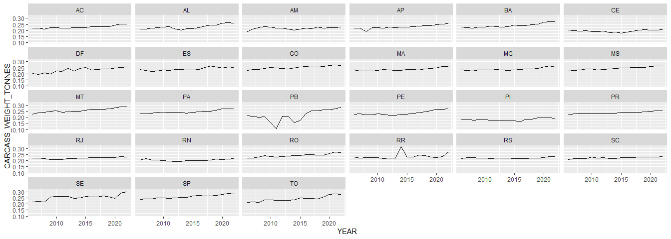
Note the years of carcass data used were 2006-2022.
Check that the trends in carcass weights make sense. Some quirks (e.g. RR in 2015, PB in 2010) but these are OK, as these states slaughter few cattle in any case.
carcass_weights %>%
  ggplot(aes(YEAR, CARCASS_WEIGHT_TONNES)) +
  geom_line() +
  facet_wrap(~STATE_ABBR)
Next, join the carcass weights to the slaughterhouse list:
# NB I pick one value per CNPJ (there are some cases where a CNPJ is registered as both an SIF and an SIE, and we take the larger slaughterhouse size).
sh_list_weights <-
  sh_heads %>%
  select(EMPRESA, ABIEC, CNPJ, NIVEL_DE_INSPECAO, LH_GEOCODE = GEOCODE, MUNICIPIO, ESTADO, TIPO, COMPROMISSOS, MEDIAN_NUM_CATTLE, HEADS, SIGNING_YEAR) %>%
  mutate(NIVEL_DE_INSPECAO = ifelse(NIVEL_DE_INSPECAO == "CONSORCIO", "SIM", NIVEL_DE_INSPECAO)) %>%
  left_join(carcass_weights, by = c("ESTADO" = "STATE_ABBR"), relationship = "many-to-many") %>%
  mutate(TONNES_PER_FACILITY = CARCASS_WEIGHT_TONNES * MEDIAN_NUM_CATTLE)


# Check the number of rows match
# ... NB we created one record per slaughterhouse/year.
stopifnot(nrow(sh_list_weights) / length(unique(carcass_weights$YEAR)) == nrow(sh_heads))
Add the supply sheds
# Load single supply shed per CNPJ8, GEOCODE
supply_sheds_cnpj8_nested <-
  s3readRDS(
  object = paste0("brazil/logistics/gta/network/BOV/SUPPLY_SHED/2024_MUNICIPAL_PER_CNPJ8/RDS/CNPJ8_SUPPLY_SHEDS.rds"),
  bucket = "trase-storage",
  opts = c("check_region" = T)
) %>%
  mutate(SOURCE = "GTA")


# Load supply shed per CNPJ8, GEOCODE, based on machine learning
# ... NB I have to standardize the names
supply_sheds_ml_nested <-
  s3read_using(
  object = paste0("brazil/logistics/gta/network/BOV/SUPPLY_SHED/2024_MUNICIPAL_PER_CNPJ8/JSON/CNPJ8_SUPPLY_SHEDS_PREDICTED.json"),
  FUN = fromJSON,
  bucket = "trase-storage",
  opts = c("check_region" = T)
) %>%
  mutate(SOURCE = "ML") %>%
  unnest() %>%
  rename(PROP_FLOWS = PRED_PROP_FLOWS_CORRECTED) %>%
  group_by(CNPJ8, LH_GEOCODE) %>%
  nest(SUPPLY_SHED = c(GEOCODE, PROP_FLOWS)) %>%
  ungroup()


# Load SIGSIF
sigsif_summary <-
  s3read_using(
    object = "brazil/production/statistics/sigsif/out/old/br_bovine_slaughter_2015_2020.csv",
    FUN = read_delim,
    col_types = cols(GEOCODE = col_character()),
    delim = ";",
    bucket = ts,
    opts = c("check_region" = T)
  ) %>%
  select(-BIOME, -QUANTITY) %>%
  group_by(STATE_SLAUGHTER) %>%
  nest(SUPPLY_SHED = c(GEOCODE, PROP_FLOWS)) %>%
  ungroup() %>%
  mutate(SOURCE = "SIGSIF")


# Add sourcing information to the slaughterhouse list
# ... where we don't have GTA-based supply sheds, we use machine learning
sh_sourcing <-
  sh_list_weights %>%
  mutate(CNPJ8 = str_sub(CNPJ, start = 1, end = 8)) %>%
  left_join(supply_sheds_cnpj8_nested, by = c("CNPJ8","LH_GEOCODE"), relationship = "many-to-one") %>%
  left_join(supply_sheds_ml_nested, by = c("CNPJ8","LH_GEOCODE"), relationship = "many-to-one", suffix = c("", "_ML")) %>%
  left_join(sigsif_summary, by = c("ESTADO" = "STATE_SLAUGHTER"), relationship = "many-to-one", suffix = c("", "_SIGSIF")) %>%
  mutate(SUPPLY_SHED = case_when(SOURCE == "GTA" ~ SUPPLY_SHED,
                                SOURCE_ML == "ML" ~ SUPPLY_SHED_ML,
                                SOURCE_SIGSIF == "SIGSIF" ~ SUPPLY_SHED_SIGSIF,
                                TRUE ~ NA)) %>%
  mutate(SUPPLY_SHED_SOURCE = coalesce(SOURCE, SOURCE_ML, SOURCE_SIGSIF)) %>%
  select(-SUPPLY_SHED_ML, -SUPPLY_SHED_SIGSIF,
         -SOURCE, -SOURCE_ML, -SOURCE_SIGSIF)


# Check no duplicates introduced during the join
stopifnot(nrow(sh_sourcing) == nrow(sh_list_weights))
Count the source of the supply shed information per slaughterhouse:
sh_sourcing %>%
  distinct(EMPRESA, CNPJ, NIVEL_DE_INSPECAO, LH_GEOCODE, SUPPLY_SHED_SOURCE) %>%
  count(SUPPLY_SHED_SOURCE)
##   SUPPLY_SHED_SOURCE   n
## 1                GTA 686
## 2                 ML 404
## 3             SIGSIF  30
## 4               <NA>   1
Which is the slaughterhouse for which no supply shed is available?
sh_sourcing %>%
  filter(is.na(SUPPLY_SHED_SOURCE)) %>%
  distinct(EMPRESA, CNPJ, NIVEL_DE_INSPECAO, TIPO, ESTADO, LH_GEOCODE)
##                             EMPRESA           CNPJ NIVEL_DE_INSPECAO
## 1 NELORE DISTRIBUIDORA DE ALIMENTOS 07112404000116               SIE
##             TIPO ESTADO LH_GEOCODE
## 1 ABATEDOURO SIE     RJ    3301108
This single case in RJ is dropped:
sh_sourcing <- sh_sourcing %>% drop_na(SUPPLY_SHED_SOURCE)
In total, this leaves us with slaughter volumes for 1120 slaughterhouses.
Calculate the slaughterhouse sourcing per municipality, per year.
sh_sourcing_sum <-
  sh_sourcing %>%
  unnest(cols = c(SUPPLY_SHED)) %>%
  mutate(SOURCED_TONNES_MUNI = PROP_FLOWS * TONNES_PER_FACILITY) %>%
  group_by(YEAR, GEOCODE) %>%
  summarise(SOURCED_TONNES_MUNI = sum(SOURCED_TONNES_MUNI, na.rm = T)) %>%
  ungroup() %>%
  mutate(YEAR = as.character(YEAR))
Compare estimated production and slaughter volumes per municipality:
sh_sourcing_sf <- prod %>%
  pivot_longer(cols = CW_PRODUCTION_TONS_2022:CW_PRODUCTION_TONS_2006, names_to = "YEAR", values_to = "CARCASS_TONNES_PRODUCTION") %>%
  mutate(YEAR = str_sub(YEAR, start = -4, end = -1),
         GEOCODE = str_sub(TRASE_ID, start = 4, end = -1)) %>%
  inner_join(sh_sourcing_sum, by = c("YEAR", "GEOCODE")) %>%
  mutate(DIFF = (CARCASS_TONNES_PRODUCTION - SOURCED_TONNES_MUNI),
         PERC_DIFF = DIFF / CARCASS_TONNES_PRODUCTION * 100) %>%
  left_join(munis, ., by = "GEOCODE") %>%
  drop_na(YEAR)


# Plot scatterplot
ggplot(sh_sourcing_sf, aes(CARCASS_TONNES_PRODUCTION, SOURCED_TONNES_MUNI)) +
  geom_point() +
  geom_abline(slope = 1, intercept = 0) +
  facet_wrap(~YEAR)
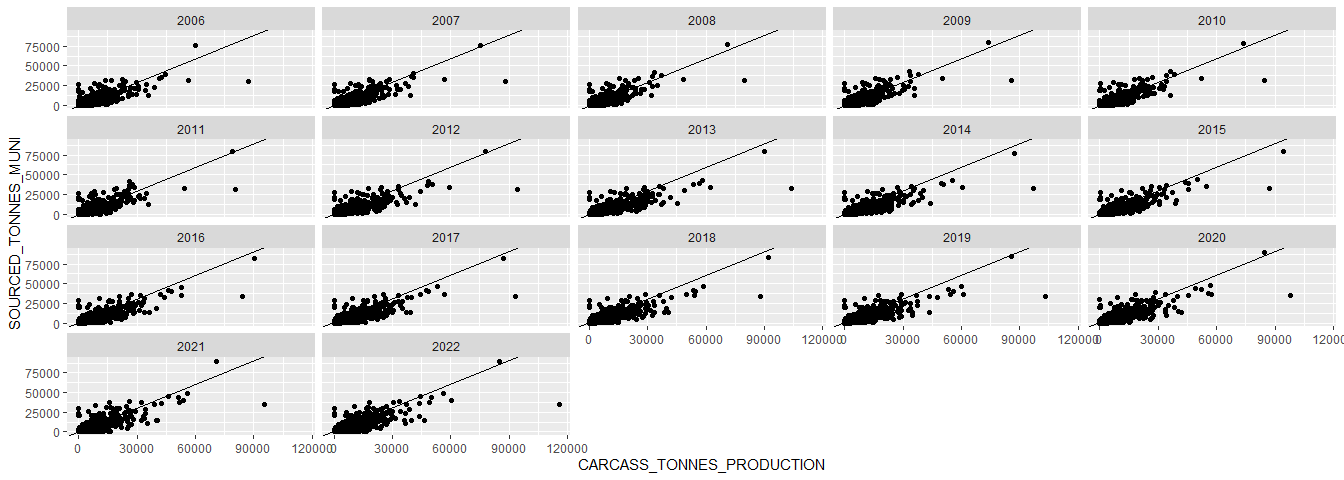
Calculate the R-sq of the relationship, just for interest:
m1 <- lm(data = sh_sourcing_sf %>% st_drop_geometry(), CARCASS_TONNES_PRODUCTION ~ SOURCED_TONNES_MUNI*as.character(YEAR))
res <- summary(m1)
res$adj.r.squared
## [1] 0.7114004
Overall our (median) estimates of registered slaughter are ~30% below the estimates of production.
sh_sourcing_total_sum <-
  sh_sourcing %>%
  unnest(cols = c(SUPPLY_SHED)) %>%
  mutate(SOURCED_TONNES_MUNI = PROP_FLOWS * TONNES_PER_FACILITY) %>%
  group_by(YEAR) %>%
  summarise(SOURCED_TONNES_MUNI = sum(SOURCED_TONNES_MUNI, na.rm = T)) %>%
  ungroup() %>%
  mutate(YEAR = as.character(YEAR))
prod %>%
  pivot_longer(cols = CW_PRODUCTION_TONS_2022:CW_PRODUCTION_TONS_2006, names_to = "YEAR", values_to = "CARCASS_TONNES_PRODUCTION") %>%
  mutate(YEAR = str_sub(YEAR, start = -4, end = -1)) %>%
  group_by(YEAR) %>%
  summarise(CARCASS_TONNES_PRODUCTION = sum(CARCASS_TONNES_PRODUCTION)) %>%
  ungroup() %>%
  inner_join(sh_sourcing_total_sum, by = c("YEAR" = "YEAR")) %>%
  mutate(PERC_DIFF = (CARCASS_TONNES_PRODUCTION - SOURCED_TONNES_MUNI) / CARCASS_TONNES_PRODUCTION * 100)
## # A tibble: 17 × 4
##    YEAR  CARCASS_TONNES_PRODUCTION SOURCED_TONNES_MUNI PERC_DIFF
##    <chr>                     <dbl>               <dbl>     <dbl>
##  1 2006                  10012419.            6212852.      37.9
##  2 2007                  10085446.            6297654.      37.6
##  3 2008                   9667164.            6346740.      34.3
##  4 2009                   9574787.            6517321.      31.9
##  5 2010                  10084619.            6560297.      34.9
##  6 2011                  10392169.            6464634.      37.8
##  7 2012                  10825757.            6491787.      40.0
##  8 2013                  11434535.            6513793.      43.0
##  9 2014                  11221615.            6522354.      41.9
## 10 2015                  10844988.            6708772.      38.1
## 11 2016                  10729179.            6803102.      36.6
## 12 2017                  10908732.            6820030.      37.5
## 13 2018                  11189777.            6832619.      38.9
## 14 2019                  11429687.            6926280.      39.4
## 15 2020                  11126117.            7158464.      35.7
## 16 2021                  10655530.            7340962.      31.1
## 17 2022                  11641584.            7300404.      37.3
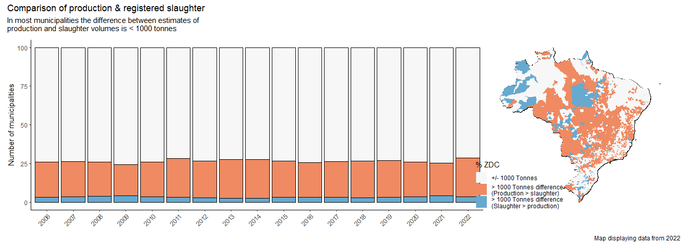
The difference is partially explained by smaller slaughterhouses, which
are not included by our data, plus uninspected slaughter, which Abiec
estimates at around 25% of all slaughter:

Note that these small +/- unregistered slaughterhouses do not have ZDCs, so the lack of data doesn’t overly affect our estimate of ZDC coverage (which we calculate as ZDC slaughter / total slaughter or production, whichever is greater).
# Visualise the spatial distribution of the mismatch production:slaughter
# NB Not sure why the legends are not being merged.
sh_sourcing_sf <- sh_sourcing_sf %>%
  mutate(DIFF_CAT = case_when(
    ((DIFF < 1000 & DIFF >= 0) | (DIFF < 0 & DIFF >= -1000)) ~ "+/- 1000 Tonnes",
    DIFF > 1000 ~ "> 1000 Tonnes difference\n(Production > slaughter)",
    DIFF < -1000 ~ "> 1000 Tonnes difference\n(Slaughter > production)",
    TRUE ~ NA_character_
    ))
p1 <- sh_sourcing_sf %>%
  st_drop_geometry() %>%
  group_by(YEAR) %>%
  mutate(N = n()) %>%
  group_by(YEAR, DIFF_CAT) %>%
  summarise(PERC_MUNIS = n() / unique(N) * 100) %>%
  ungroup() %>%
  ggplot(aes(YEAR, PERC_MUNIS, fill = DIFF_CAT)) +
  geom_bar(stat = "identity", col = "black") +
  theme_classic() +
  theme(axis.text.x = element_text(angle = 45, hjust = 1),
        axis.title.x = element_blank(),
        legend.position = "none") +
  scale_fill_manual(values = c("#f7f7f7","#ef8a62","#67a9cf")) +
  labs(y = "Number of municipalities")
p2 <- ggplot() +
  geom_sf(data = brazil, col = "black") +
  geom_sf(data = sh_sourcing_sf %>% filter(YEAR == 2022),
          aes(fill = DIFF_CAT), col = NA) +
  coord_sf(datum = NA) +
  theme_minimal() +
  theme(axis.text = element_blank(),
        legend.position = c(0.15, 0.15)) +
  scale_fill_manual(values = c("#f7f7f7","#ef8a62","#67a9cf"), name = "% ZDC")
p1 + p2 + plot_annotation(title = "Comparison of production & registered slaughter",
                          subtitle = 'In most municipalities the difference between estimates of\nproduction and slaughter volumes is < 1000 tonnes',
                   caption = "Map displaying data from 2022")
ZDC coverage is implemented as follows:
- TAC commitments cover slaughter from municipalities in the Brazilian Legal Amazon. The data on TAC signatories (company, year) come from the Boi na Linha initiative.
- The G4 was signed by JBS, Marfrig, and Minerva in 2009 and covers the Amazon, and also their subsidiary companies (e.g. PAMPEANO ALIMENTOS S/A is a subsidiary of Marfrig and covered by their commitment.)
- We include nationwide zero-coversion company commitments from Frigol (2020) and Mataboi Alimentos (rebranded as Prima Foods) who had a comprehensive ZDC from 2018 onwards (in theory).
- JBS and Marfrig set zero conversion targets in the Cerrado but with a 2025/20230 timeline, and so they are not yet covered by this time series data.
- The Cerrado Protocol was only announced in 2024, and is not yet implemented at time of writing. (And so not captured here either).
- When calculating the ZDC market share we divide the tonnes sourced per municipality under ZDCs by the total slaughter or production tonnes, whichever is larger.
# Load Trase's company commitment data, just for reference
# ... Looking at it more closely, it's a bit of a mess
# ... E.g. having Marfrig down with a nationwide commitment since 2009 (which is not true)
# ... And JBS with a nationwide commitment in 2019...?
# company_commitments <- s3read_using(
#   object = "world/indicators/actors/zdc/in/ZDC data collection 2023 vs2.xlsx",
#   bucket = "trase-storage",
#   FUN = read_xlsx,
#   opts = c("check_region" = T)
# )
# company_commitments %>% filter(Country == "Brazil", Commodity == "Beef", ZDC_FLAG != "TAC", ZDC_FLAG != "None") %>% distinct(trase_id, Exporter, Year, ZDC_FLAG, BIOME, YEAR_START) %>% as.data.frame()


# Add the ZDC column (1/0) whether or not sourcing is covered buy a commitment
# ... and then calculate `ZDC_TONNES`
# NB: As part of the calculation of sourcing sheds, (very) small volumes identified in the GTA are aggregated -> E.g. "AGGREGATED ALAGOAS"
# ... here these are dropped from the calculation (as the municipality of origin isn't known).
zdc_sourcing_sum <-
  sh_sourcing %>%
  unnest(cols = c(SUPPLY_SHED)) %>%
  select(-BIOME) %>%
  left_join(muni_biomes, by = "GEOCODE") %>%
  drop_na(BIOME) %>%
  mutate(SOURCED_TONNES_MUNI = PROP_FLOWS * TONNES_PER_FACILITY) %>%
  mutate(ZDC = case_when(
    # G4
    grepl("JBS|MINERVA|MARFRIG", EMPRESA) & YEAR >= 2009 & BIOME == "AMAZON" ~ "G4",
    # Company commitments
    EMPRESA == "PRIMA FOODS" & YEAR >= 2018 ~ "COMPANY COMMITMENT",
    EMPRESA == "FRIGOL" & YEAR >= 2020 ~ "COMPANY COMMITMENT",
    # Slaughterhouses without TAC
    is.na(SIGNING_YEAR) ~ "NONE",
    # TAC
    YEAR >= SIGNING_YEAR & GEOCODE %in% bla ~ "TAC",
    # The rest
    .default = "NONE")
    ) %>%
  group_by(YEAR, GEOCODE, ZDC) %>%
  summarise(SUM_SOURCED_TONNES = sum(SOURCED_TONNES_MUNI, na.rm = T)) %>%
  ungroup() %>%
  pivot_wider(names_from = ZDC, values_from = SUM_SOURCED_TONNES, values_fill = 0) %>%
  mutate(TOTAL_SLAUGHTER_TONNES = NONE + G4 + TAC + `COMPANY COMMITMENT`,
         ZDC_TONNES  = G4 + TAC + `COMPANY COMMITMENT`) %>%
  select(YEAR, GEOCODE,  G4, TAC, `COMPANY COMMITMENT`, ZDC_TONNES, TOTAL_SLAUGHTER_TONNES) %>%
  mutate(YEAR = as.character(YEAR))


# Add in the municipal cattle production data
zdc_market_share <-
  prod %>%
  pivot_longer(cols = CW_PRODUCTION_TONS_2022:CW_PRODUCTION_TONS_2006, names_to = "YEAR", values_to = "CARCASS_TONNES_PRODUCTION") %>%
  mutate(YEAR = str_sub(YEAR, start = -4, end = -1),
         GEOCODE = str_sub(TRASE_ID, start = 4, end = -1)) %>%
  filter(CARCASS_TONNES_PRODUCTION > 0) %>%
  select(-TRASE_ID) %>%
  full_join(zdc_sourcing_sum, by = c("YEAR", "GEOCODE")) %>%
  mutate(CARCASS_TONNES_PRODUCTION= replace_na(CARCASS_TONNES_PRODUCTION, 0),
         G4 = replace_na(G4, 0),
         TAC = replace_na(TAC, 0),
         `COMPANY COMMITMENT` = replace_na(`COMPANY COMMITMENT`, 0),
         TOTAL_SLAUGHTER_TONNES = replace_na(TOTAL_SLAUGHTER_TONNES, 0),
         ZDC_TONNES = replace_na(ZDC_TONNES, 0),
         PROP_ZDC = case_when(
           (ZDC_TONNES > CARCASS_TONNES_PRODUCTION) & (ZDC_TONNES > TOTAL_SLAUGHTER_TONNES) ~ 1,
           TOTAL_SLAUGHTER_TONNES >= CARCASS_TONNES_PRODUCTION ~ ZDC_TONNES / TOTAL_SLAUGHTER_TONNES,
           TOTAL_SLAUGHTER_TONNES < CARCASS_TONNES_PRODUCTION ~ ZDC_TONNES / CARCASS_TONNES_PRODUCTION,
           .default = NA_real_))
stopifnot(any(is.na(zdc_market_share$PROP_ZDC)) == F)
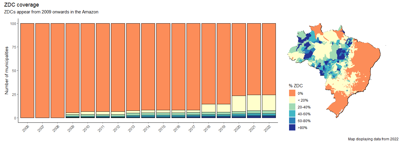
Visualise the ZDC marketshare
# NB we drop two municipalties in the Pampa with zero cattle production (4300001, 4300002)
zdc_market_share_sf <- zdc_market_share %>%
  # Fix this
  mutate(PERC_ZDC_CAT = case_when(
    PROP_ZDC == 0 ~ "0%",
    PROP_ZDC <= 0.20 ~ "< 20%",
    PROP_ZDC <= 0.40 ~ "20-40%",
    PROP_ZDC <= 0.60 ~ "40-60%",
    PROP_ZDC <= 0.80 ~ "60-80%",
    PROP_ZDC <= 1.0 ~ ">80%",
    TRUE ~ NA_character_),
    PERC_ZDC_CAT = as_factor(PERC_ZDC_CAT),
    PERC_ZDC_CAT = fct_relevel(PERC_ZDC_CAT, c("0%", "< 20%", "20-40%", "40-60%", "60-80%", ">80%"))) %>%
  left_join(munis, ., by = "GEOCODE") %>%
  drop_na(YEAR) %>%
  filter(CARCASS_TONNES_PRODUCTION > 0)
p1 <- zdc_market_share_sf %>%
  st_drop_geometry() %>%
  group_by(YEAR) %>%
  mutate(N = n()) %>%
  group_by(YEAR, PERC_ZDC_CAT) %>%
  summarise(PERC_MUNIS = n() / unique(N) * 100) %>%
  ungroup() %>%
  ggplot(aes(YEAR, PERC_MUNIS, fill = PERC_ZDC_CAT)) +
  geom_bar(stat = "identity", col = "black") +
  theme_classic() +
  theme(axis.text.x = element_text(angle = 45, hjust = 1),
        axis.title.x = element_blank(),
        legend.position = "none") +
  scale_fill_manual(values = c("#fc8d59", "#ffffcc", "#a1dab4", "#41b6c4", "#2c7fb8", "#253494")
) +
  labs(y = "Number of municipalities")
p2 <- ggplot() +
  geom_sf(data = brazil, col = "black") +
  geom_sf(data = zdc_market_share_sf %>% filter(YEAR == 2022),
          aes(fill = PERC_ZDC_CAT), col = NA) +
  coord_sf(datum = NA) +
  theme_minimal() +
  theme(axis.text = element_blank(),
        legend.position = c(0.15, 0.15)) +
  scale_fill_manual(values = c("#fc8d59", "#ffffcc", "#a1dab4", "#41b6c4", "#2c7fb8", "#253494"), name = "% ZDC") +
  NULL
p1 + p2 +
   plot_annotation(title = "ZDC coverage", subtitle = 'ZDCs appear from 2009 onwards in the Amazon',
                   caption = "Map displaying data from 2022")
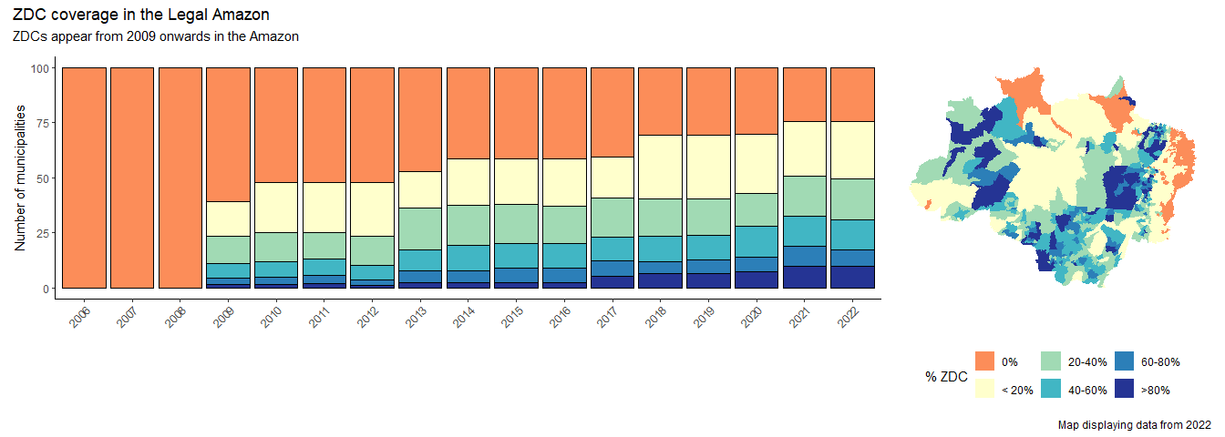
Replot the above, but zooming in on the Amazon.
p1 <- zdc_market_share_sf %>%
  st_drop_geometry() %>%
  filter(GEOCODE %in% bla) %>%
  group_by(YEAR) %>%
  mutate(N = n()) %>%
  group_by(YEAR, PERC_ZDC_CAT) %>%
  summarise(PERC_MUNIS = n() / unique(N) * 100) %>%
  ungroup() %>%
  ggplot(aes(YEAR, PERC_MUNIS, fill = PERC_ZDC_CAT)) +
  geom_bar(stat = "identity", col = "black") +
  theme_classic() +
  theme(axis.text.x = element_text(angle = 45, hjust = 1),
        axis.title.x = element_blank(),
        legend.position = "none") +
  scale_fill_manual(values = c("#fc8d59", "#ffffcc", "#a1dab4", "#41b6c4", "#2c7fb8", "#253494")
) +
  labs(y = "Number of municipalities")
p2 <- ggplot() +
  # geom_sf(data = brazil, col = "black") +
  geom_sf(data = zdc_market_share_sf %>% filter(YEAR == 2022, GEOCODE %in% bla),
          aes(fill = PERC_ZDC_CAT), col = NA) +
  coord_sf(datum = NA) +
  theme_minimal() +
  theme(axis.text = element_blank(),
        legend.position = "bottom") +
  scale_fill_manual(values = c("#fc8d59", "#ffffcc", "#a1dab4", "#41b6c4", "#2c7fb8", "#253494"), name = "% ZDC") +
  NULL
p1 + p2 +
   plot_annotation(title = "ZDC coverage in the Legal Amazon", subtitle = 'ZDCs appear from 2009 onwards in the Amazon',
                   caption = "Map displaying data from 2022")
This could also be plotted as % of production (rather than the number of municipalities).
Export the data
Data exported with the following fields:
YEARGEOCODE- IBGE code of the municipalityBIOME- Biome of the municipalityPRODUCTION_TONNES- Live carcass weight tonnes/municipality/yearZDC_TONNES- the tonnes slaughtered in ZDC slaughterhousesPROP_ZDC- the proportion (0-1) slaughtered in ZDC slaughterhouses
# Note I simplify the data to a single production column
# ... whichever is greater, production or registered slaughter
zdc_market_share_sf %>%
  st_drop_geometry() %>%
  mutate(PRODUCTION_TONNES = ifelse(CARCASS_TONNES_PRODUCTION > TOTAL_SLAUGHTER_TONNES, CARCASS_TONNES_PRODUCTION, TOTAL_SLAUGHTER_TONNES)) %>%
  select(YEAR, GEOCODE, BIOME, PRODUCTION_TONNES, G4, TAC, `COMPANY COMMITMENT`, ZDC_TONNES, PROP_ZDC) %>%
  s3write_using(
    x = .,
    object = "brazil/beef/analysis/zdc_coverage_2006_2022.csv",
    bucket = "trase-storage",
    FUN = write_delim,
    delim = ";"
  )
Cross-check variation in slaughter estimates
The above calculation is done using the median slaughterhouse sizes estimates (per category of slaughterhouse) to calculate ZDC marketshare.
Here I include code just to cross check these ‘median’ estimates against other national-level data sources (Abiec statistics and our production estimate for the country).
# CHECK AGAINST OTHER SCRIPTS ESTIMATING SLAUGHTER VOLUMES
# Code adapated from scripts/PESQUISA/SLAUGHTER/ESTIMATE_NATIONAL_SLAUGHTER_VOLUME.md

# Load slaughterhouse sizes
# ... loaded again to get the full Monte-Carlo sample
sh_sizes <- s3read_using(
  object = "data/SLAUGHTER/slaughterhouse_sizes_mc/2024-07-04-monte_carlo_sh_size.csv",
  delim = ";",
  bucket = "trase-app",
  FUN = read_delim
) %>%
  group_by(TYPE) %>%
  nest(HEADS = c(NUM_CATTLE, ITERATION)) %>%
  ungroup()


# Get 10000 samples of the carcass weight per state
n_iterations <- 10000
carcass_weights_mc <- carcass_weights %>%
  group_by(STATE_NAME, STATE_ABBR) %>%
  sample_n(size = n_iterations, replace = T) %>%
  mutate(ITERATION = row_number()) %>%
  ungroup() %>%
  select(STATE_ABBR, CARCASS_WEIGHT_TONNES, ITERATION)


# Join slaughterhouse sizes to the slaughterhouse list
sh_with_sizes <- ind %>%
  mutate(ABIEC = case_when(EMPRESA %in% abiec ~ "ABIEC",
                           TRUE ~ "FRIGORÍFICOS\nNÃO ASSOCIADOS")) %>%
  left_join(sh_sizes, by = c("TIPO" = "TYPE", "ABIEC"))


# Join the carcass weights to the slaughterhouse list
# ... and calculate deforestation risk
# ... also shorten company names
# ... NB I pick one value per CNPJ (there are some cases where a CNPJ is registered as both an SIF and an SIE, and we take the larger slaughterhouse size).
sh_with_sizes_mc <-
  sh_with_sizes %>%
  mutate(EMPRESA = case_when(EMPRESA == "INDUSTRIA E COMERCIO DE CARNES E DERIVADOS BOI BRASIL" ~ "BOI BRASIL",
                             EMPRESA == "COOPERATIVA DOS PRODUTORES DE CARNE E DERIVADOS DE GURUPI" ~ "COOPERFRIGU",
                             grepl("MARFRIG", EMPRESA) ~ "MARFRIG",
                             EMPRESA == "HIPERCARNES INDUSTRIA E COMERCIO" ~ "HIPERCARNES",
                             EMPRESA == "MAPPISA INDUSTRIA E COMERCIO DE CARNES" ~ "FRIGORIFICO MAPPI",
                             EMPRESA == "FRIBARREIRAS AGRO INDUSTRIAL DE ALIMENTOS" ~ "FRIBARREIRAS",
                             EMPRESA == "NACIONAL DISTRIBUIDORA DE CARNES BEEF" ~ "BEEF NOBRE",
                             EMPRESA == "PANTANEIRA INDUSTRIA E COMERCIO DE CARNES E DERIVADOS" ~ "PANTANEIRA",
                             EMPRESA == "INDUSTRIA E COMERCIO DE ALIMENTOS SUPREMO" ~ "SUPREMO CARNES",
                             EMPRESA == "SF INDUSTRIA E COMERCIO DE CARNES" ~ "FRIGORIFICO RIO CLARO",
                             EMPRESA == "BRASIL GLOBAL AGROINDUSTRIAL" ~ "BRASIL GLOBAL",
                             EMPRESA == "AGRA AGROINDUSTRIAL DE ALIMENTOS" ~ "AGRA FOODS",
                             TRUE ~ EMPRESA)) %>%
  filter(EMPRESA != "COORDENACAO DE LABORATORIO ANIMAL") %>%
  unnest(cols = c("HEADS")) %>%
  left_join(carcass_weights_mc, by = c("ESTADO" = "STATE_ABBR", "ITERATION")) %>%
  mutate(TOTAL_CARCASS_TONNES = CARCASS_WEIGHT_TONNES * NUM_CATTLE) %>%
  group_by(EMPRESA, ABIEC, CNPJ, NIVEL_DE_INSPECAO, GEOCODE, MUNICIPIO, ESTADO, TIPO) %>%
  mutate(MEDIAN_TONNES = quantile(TOTAL_CARCASS_TONNES, probs = 0.5)) %>%
  group_by(EMPRESA, ABIEC, CNPJ, NIVEL_DE_INSPECAO, GEOCODE, MUNICIPIO, ESTADO, TIPO, MEDIAN_TONNES) %>%
  nest() %>%
  group_by(CNPJ) %>%
  filter(MEDIAN_TONNES == max(MEDIAN_TONNES)) %>%
  ungroup()


# ABIEC
# ... data from Abiec's annual reports
abiec_estimates <- tribble(
  ~YEAR, ~TOTAL, ~PRODUCT_SIMPLE,
  "2022", 9.7 * 1e06, "BEEF",
) %>%
  mutate(SOURCE = "ABIEC")


# Estimate of cattle production
prod_summary <-
  prod %>%
  pivot_longer(cols = CW_PRODUCTION_TONS_2022:CW_PRODUCTION_TONS_2006, names_to = "YEAR", values_to = "CW_PRODUCTION_TONS") %>%
  mutate(YEAR = str_sub(YEAR, start = -4, end = -1)) %>%
  group_by(YEAR) %>%
  summarise(TOTAL = sum(CW_PRODUCTION_TONS)) %>%
  ungroup() %>%
  filter(YEAR %in% "2022") %>%
  mutate(SOURCE = "NATIONAL PRODUCTION\nESTIMATE")


# Visualise the comparison of our slaughter estimate vs Abiec's
sh_with_sizes_mc %>%
  unnest(cols = c(data)) %>%
  group_by(ITERATION) %>%
  summarise(TOTAL_SLAUGHTER_TONNES = sum(TOTAL_CARCASS_TONNES)) %>%
  ungroup() %>%
  summarise(TOTAL = quantile(TOTAL_SLAUGHTER_TONNES, probs = 0.5),
            Q975 = quantile(TOTAL_SLAUGHTER_TONNES, probs = 0.975),
            Q025 = quantile(TOTAL_SLAUGHTER_TONNES, probs = 0.025),
            Q90 = quantile(TOTAL_SLAUGHTER_TONNES, probs = 0.9),
            Q10 = quantile(TOTAL_SLAUGHTER_TONNES, probs = 0.1),
            Q33 = quantile(TOTAL_SLAUGHTER_TONNES, probs = 0.33),
            Q66 = quantile(TOTAL_SLAUGHTER_TONNES, probs = 0.66)) %>%
  ungroup() %>%
  mutate(SOURCE = "ABATE TOTAL") %>%
  bind_rows(abiec_estimates, prod_summary) %>%
  mutate(YEAR = as.character(YEAR)) %>%
  ggplot(aes(SOURCE, TOTAL)) +
  geom_bar(stat = "identity", position = "dodge") +
  geom_errorbar(aes(ymin = Q10, ymax = Q90), width = 0) +
  geom_errorbar(aes(ymin = Q33, ymax = Q66), width = 0, linewidth = 1.2) +
  theme_classic() +
  ylab("Carne bovina\n(Toneladas de carçaca)") +
  labs(title = "Estimates of total carcass weight (2022 data)",
       subtitle = "Our median slaughter estimate is a bit less than Abiec, which is smaller than the national production.\nWhich makes sense, as Abiec's estimate should cover more slaughterhouses than our list (which is incomplete\nand the Abiec data here doesn't include informal slaughter.") +
  scale_y_continuous(label = unit_format(unit = "M", scale = 1e-6, sep = ""))

Finally, double-check the comparison of the median tonnes/facility as estimated early on in this script vs the end. The two figures are very similar, phew. :)
# Compare median tonnes/facility
# ... small difference
sh_with_sizes_mc %>%
  select(CNPJ, MEDIAN_TONNES) %>%
  summarise(SUM_MEDIAN_TONNES = sum(MEDIAN_TONNES))
## # A tibble: 1 × 1
##   SUM_MEDIAN_TONNES
##               <dbl>
## 1          6750896.
sh_list_weights %>%
  drop_na(TONNES_PER_FACILITY) %>%
  group_by(CNPJ, NIVEL_DE_INSPECAO, LH_GEOCODE) %>%
  summarise(MEDIAN_TONNES_MC = quantile(TONNES_PER_FACILITY, 0.5)) %>%
  ungroup() %>%
  summarise(SUM_MEDIAN_TONNES_MC = sum(MEDIAN_TONNES_MC))
## # A tibble: 1 × 1
##   SUM_MEDIAN_TONNES_MC
##                  <dbl>
## 1             6606702.