Cattle production data 2010-2022
Erasmus zu Ermgassen 31/01/2024
This script calculates cattle production (ton carcass) per municipality, per year (2024-01-31-CATTLE_PRODUCTION_5_YR.csv).
This is calculated as the herd size (per muni/yr) * slaughter rate (per state/yr) * carcass weight (per state/yr)
Herd size data
From the PPM.
# Load PPM data
ppm <- s3read_using(
  object = "brazil/production/statistics/ibge/cattle/ppm/out/PPM_BOV_HERD_1974_2022.csv",
  FUN = read_delim,
  delim = ";",
  bucket = "trase-storage",
  col_types = cols(GEOCODE = col_character()),
  opts = c("check_region" = T)
) %>%
  mutate(TWO_DIGIT_CODE = str_sub(GEOCODE, start = 1, end = 2)) %>%
  left_join(state_dic, by = "TWO_DIGIT_CODE") %>%
  rename(STATE = STATE_NAME)
The slaughter rate
The slaughter (or offtake) rate is calculated from the number of cattle per state / the number cattle slaughtered per state.
The number cattle slaughtered per state is calculated in the following way:
- We use Anualpec data on slaughtered head per state (2011-2021). We favour these over the IBGE slaughter survey, because they are more complete (they include all slaughterhouses in theory, including informal slaughter).
- The Anualpec timeseries is extended to other years by calculating the mean difference between the Anualpec and IBGE slaughter statistics (which are available for more years) per state, and then correcting the IBGE slaughter statistics from pre-2011 (where Anualpec is not available).
- These slaughter numbers are the number of animals slaughtered IN a state - animals may of course be slaughtered in a different state from where they are raised. We correct for this using SIGSIF data on cattle movements to SIF slaughterhouses, adding/subtracting the number of cattle head recorded as moving from/to each state. This misses inter-state movements to other (SIE/SIM) slaughterhouses, though these inter-state movements are likely to be an order of magnitude less common than movements to SIF slaughterhouses. The SIGSIF data were only available for 2015-2021; we correct previous years slaughter data, assuming the same proportion of slaughter movements are inter-state as in later years.
- Finally, the slaughter number is divided by the annual state herd size to estimate the slaughter rate per state per year.
- Carcass weights are calculated per state from IBGE statistics.
- Finally, the herd size (PPM), slaughter rate (composite), and carcass weight (IBGE) are multiplied to estimate production.
- The production is reported both on an annual (
CW_PRODUCTION_TONS) and lifecycle (CW_PRODUCTION_TONS_5_YR) basis.
Slaughter data
# Load anualpec abate (slaughter) data
aa <-
  s3read_using(
  object = "brazil/production/statistics/anualpec/out/ANUALPEC_BOV_ABATE_2021.csv",
  FUN = read_delim,
  delim = ";",
  bucket = "trase-storage",
  opts = c("check_region" = T)
)


# Load 2019 data, since this also has 2011
aa_2019 <- s3read_using(
  object = "brazil/production/statistics/anualpec/out/ANUALPEC_BOV_ABATE_2019.csv",
  FUN = read_delim,
  delim = ";",
  bucket = "trase-storage",
  opts = c("check_region" = T)
) %>%
  filter(YEAR == 2011)


# Join Anualpec time series together
aa <- bind_rows(aa, aa_2019)
rm(aa_2019)
NB I chose the Anualpec data because it is more complete than the IBGE trimestral survey, e.g. including estimates for informal slaughterhouses. This is shown below.
# Compare Anualpec & IBGE survey


# Load IBGE survey
ibge_abate <-
  s3read_using(
    object = "brazil/production/statistics/ibge/cattle/carcass_weights/IN/tabela1092.csv",
    delim = ";",
    FUN = read_delim,
    skip = 3,
    bucket = "trase-storage",
    opts = c("check_region" = T)
  ) %>%
  slice(-1) %>%
  janitor::clean_names("screaming_snake") %>%
  mutate(
    YEAR = as.numeric(str_sub(TRIMESTRE, start = 14, end = 17)),
    ANIMAIS_ABATIDOS_CABECAS = as.numeric(ANIMAIS_ABATIDOS_CABECAS)
  ) %>%
  mutate(STATE = str_trans(UNIDADE_DA_FEDERACAO)) %>%
  group_by(STATE, YEAR) %>%
  summarise(NUM_HEAD = sum(ANIMAIS_ABATIDOS_CABECAS, na.rm = T)) %>%
  ungroup() %>%
  filter(!is.na(YEAR))


# Plot comparison of the datasets
years_in_both <- intersect(aa$YEAR, ibge_abate$YEAR)
comp_ibge_aa <- bind_rows(aa, ibge_abate, .id = "DATA_SOURCE") %>%
  mutate(DATA_SOURCE = ifelse(DATA_SOURCE == "1", "ANUALPEC","IBGE")) %>%
  filter(YEAR %in% years_in_both)
comp_ibge_aa %>%
  ggplot(aes(YEAR, NUM_HEAD/1e06, fill = DATA_SOURCE)) +
  geom_bar(stat = "identity", position = "dodge") +
  theme_bw() +
  facet_wrap(~STATE, scales = "free_y", ncol = 7) +
  theme(legend.position = c(0.93,0.08),
        legend.title = element_blank(),
        axis.title.x = element_blank()) +
  scale_y_continuous(label = unit_format(unit = "M")) +
  ylab("Number of cattle slaughtered") +
  geom_hline(yintercept = 0) +
  scale_fill_manual(values = c("#0072B2", "#D55E00"))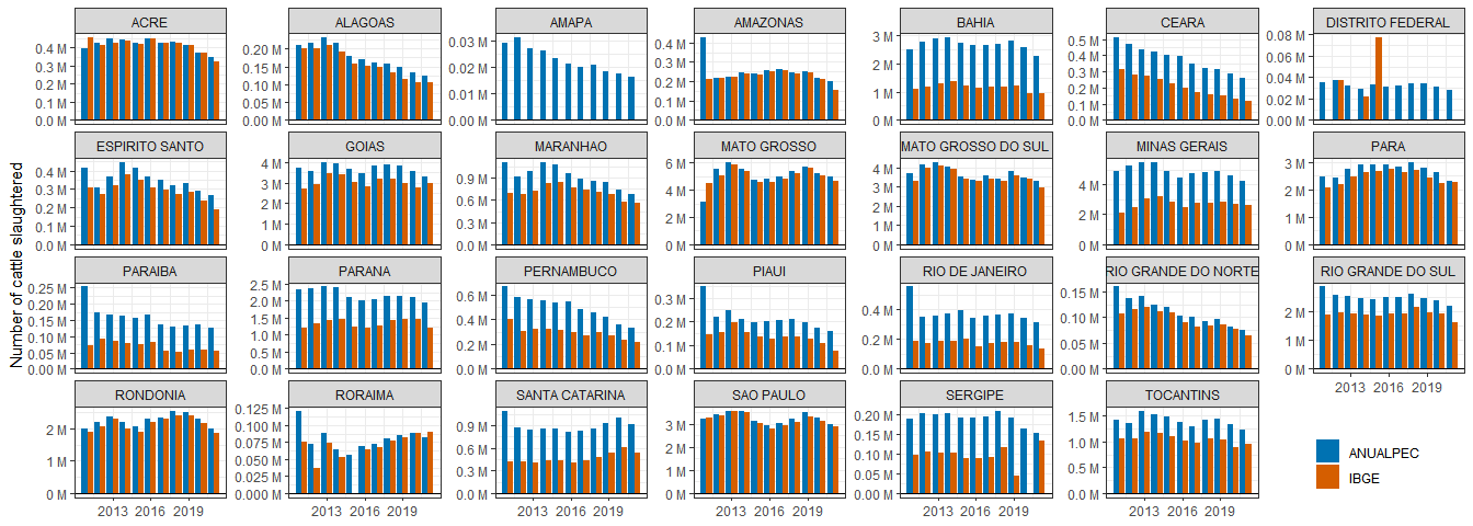
We however want a longer slaughter time series of slaughter (covering 2006-2019, for SEI-PCS 2010-2019) than available from Anualpec (2011-2021 only).
We therefore interpolate the difference between the Anualpec and IBGE data, for those earlier years (pre-2011) where we don’t have Anualpec slaughter statistics.
First we plot the consistency of the difference (Anualpec vs IBGE) over time.
# Calculate the % difference between IBGE and Anualpec per state
perc_diff <-
  comp_ibge_aa %>%
  select(-STATE_ABBR) %>%
  spread(DATA_SOURCE, NUM_HEAD) %>%
  mutate(PERC_DIFF = (ANUALPEC - IBGE) / IBGE * 100)


# Visualise the difference
perc_diff %>%
  ggplot(aes(STATE, PERC_DIFF, col = YEAR)) +
  geom_boxplot() +
  geom_point() +
  theme_minimal() +
  coord_flip()
Wide variation in "SE","PE","RR", "PB", "DF","CE","AP".
There is small uncertainty within states, except for SE, RR, PE, PB, DF, CE, and AP. These states made up a cumulative 3% of slaughter (2011-2021), and therefore this uncertainty doesn’t affect the overall calculation much.
We therefore ‘correct’ the IBGE statistics for each state, using the mean difference between IBGE and Anualpec (2011-2019) to estimate the slaughter in earlier (pre-2011) and later (2022-2023) where Anualpec is not available, but IBGE is.
For some state/years, the IBGE data were missing. In these cases we used the mean number of cattle per state (from IBGE) available for other years. Finally, for Amapa, no IBGE data were available post-2010 (but they ); we therefore used the mean IBGE slaughter numbers from other years to approximate slaughter volumes.
i.e. slaughter heads = ibge * correction factor.
# Interpolate the 'anualpec' data for previous years
# ... based on the relationship in years where both datasets exist.
# ... Note: we exclude outliers (AM in 2011 & DF in 2015) from the calculation of the correction factor


# Identify the correction factor
corr_factor <-
  perc_diff %>%
  filter(
    !(STATE == "AMAZONAS" & YEAR == 2011),
      !(STATE == "DISTRITO FEDERAL" & YEAR == 2015)
    ) %>%
  filter(PERC_DIFF != Inf) %>%
  group_by(STATE) %>%
  summarise(CORRECTION_FACTOR = 1 + mean(PERC_DIFF, na.rm = T) / 100) %>%
  ungroup()


# Identify the values to 'gap fill'
fill_ibge_gap <-
  ibge_abate %>%
  filter(NUM_HEAD != 0) %>%
  group_by(STATE) %>%
  summarise(NUM_HEAD_GAP_FILL = mean(NUM_HEAD, na.rm = T))
ap_mean <-
  aa %>% filter(STATE == "AMAPA") %>%
  summarise(MEAN_NUM_HEAD = mean(NUM_HEAD)) %>%
  ungroup() %>%
  pull(MEAN_NUM_HEAD)
aa_corrected <- full_join(aa, ibge_abate, by = c("STATE", "YEAR"), suffix = c("_ANUALPEC", "_IBGE")) %>%
  left_join(fill_ibge_gap, by = "STATE") %>%
  mutate(NUM_HEAD_IBGE = case_when(NUM_HEAD_IBGE == 0 ~ NUM_HEAD_GAP_FILL,
                                       TRUE ~ NUM_HEAD_IBGE)) %>%
  left_join(corr_factor, by = "STATE") %>%
  mutate(NUM_HEAD_ANUALPEC = case_when(is.na(NUM_HEAD_ANUALPEC) & !is.na(CORRECTION_FACTOR) ~ NUM_HEAD_IBGE * CORRECTION_FACTOR,
                                       is.na(NUM_HEAD_ANUALPEC) & is.na(CORRECTION_FACTOR) ~ NUM_HEAD_IBGE,
                                       TRUE ~ NUM_HEAD_ANUALPEC)) %>%
  select(
    STATE,
    YEAR,
    NUM_HEAD = NUM_HEAD_ANUALPEC
  )
stopifnot(all(aa_corrected$NUM_HEAD != 0))
Below we check that these ‘corrected’ time series look reasonable:
aa_corrected %>%
  ggplot(aes(YEAR, NUM_HEAD)) +
  facet_wrap(~STATE) +
  geom_line() +
  theme_minimal() +
  theme(axis.text.x = element_text(angle = 45, hjust = 1),
        axis.title.x = element_blank()) +
  ylab("Number of cattle slaughtered/year") +
  labs(title = "Slaughter time series, correcting for IBGE:Anualpec gap")
Since we are interested in calculating production per municipality (and state), but the slaughter data include the ‘import’ of cattle from other states, we correct for inter-state movements of cattle to slaughter (which are by default included in Anualpec and the IBGE slaughter data), using data on inter-state slaughter movements reported in SIGSIF.
# Calculate the proportion of SIF slaughter per state that is inter-state


# [A] Load raw SIGSIF for 2015-2019
# Note: these data are semi_colon delimted
path <- "brazil/production/statistics/sigsif/out/"
keys <- map_chr(get_bucket(ts, prefix = path), "Key")
keys_semi_colon <- keys[grepl("SIF_2015_2017|SIF_2018|SIF_2019", keys)]
keys_semi_colon <- keys_semi_colon[grepl("csv", keys_semi_colon)]
sigsif_2015_2019 <-
  map_df(keys_semi_colon,
         ~ s3read_using(
           object = .x,
           FUN = read_delim,
           col_types = cols(GEOCODE = col_character()),
           delim = ";",
           bucket = ts,
           opts = c("check_region" = T)
         )
  )


# [B] Load raw SIGSIF for 2020 and 2021
# Note: these data are comma delimted
keys_comma <- keys[grepl("SIF_2020|SIF_2021", keys)]
keys_comma <- keys_comma[grepl("csv", keys_comma)]
sigsif_2020_2021 <-
  map_df(keys_comma,
         ~ s3read_using(
           object = .x,
           FUN = read_delim,
           col_types = cols(GEOCODE = col_character()),
           delim = ";",
           bucket = ts,
           opts = c("check_region" = T)
         )
  )


# [C] Join 2015-2021 data together
sigsif <- bind_rows(sigsif_2015_2019, sigsif_2020_2021)


# Fix missing GEOCODEs
# ... filter to cattle
sigsif <- sigsif %>%
  filter(TYPE == "CATTLE") %>%
  mutate(GEOCODE = case_when(
    is.na(GEOCODE) & MUNICIPALITY == "MIRASSOL D OESTE" ~ "5105622",
    TRUE ~ GEOCODE
  ))
stopifnot(any(is.na(sigsif$GEOCODE)) == FALSE)


# tidy up
rm(sigsif_2015_2019, sigsif_2020_2021, path, keys, keys_comma, keys_semi_colon)


# (A) slaughter per DESTINATION state where cattle originate from inter-state movements
sigsif_dest <-
  sigsif %>%
  mutate(TWO_DIGIT_CODE = str_sub(GEOCODE, start = 1, end = 2)) %>%
  left_join(state_dic, by = "TWO_DIGIT_CODE") %>%
  rename(STATE_ORIGIN = STATE_ABBR) %>%
  select(-STATE_NAME) %>%
  mutate(INTER_STATE_MOVEMENT = ifelse(STATE_SLAUGHTER == STATE_ORIGIN, F, T)) %>%
  filter(INTER_STATE_MOVEMENT == T) %>%
  group_by(YEAR, STATE_SLAUGHTER) %>%
  summarise(NUM_HEAD_ARRIVING_FOR_SLAUGHTER = sum(QUANTITY)) %>%
  ungroup()


# (B) Number of SIF-slaughtered cattle per ORIGIN state, where cattle slaughtered inter-state
sigsif_orgn <-
  sigsif %>%
  mutate(TWO_DIGIT_CODE = str_sub(GEOCODE, start = 1, end = 2)) %>%
  left_join(state_dic, by = "TWO_DIGIT_CODE") %>%
  rename(STATE_ORIGIN = STATE_ABBR) %>%
  select(-STATE_NAME) %>%
  mutate(INTER_STATE_MOVEMENT = ifelse(STATE_SLAUGHTER == STATE_ORIGIN, F, T)) %>%
  filter(INTER_STATE_MOVEMENT == T) %>%
  group_by(YEAR, STATE_ORIGIN) %>%
  summarise(NUM_HEAD_SENT_FOR_SLAUGHTER = sum(QUANTITY)) %>%
  ungroup()


# (C) Join these together
slaughter <-
  left_join(aa_corrected, state_dic, by = c("STATE" = "STATE_NAME")) %>%
  select(-TWO_DIGIT_CODE) %>%
  full_join(sigsif_dest, by = c("STATE_ABBR" = "STATE_SLAUGHTER", "YEAR")) %>%
  full_join(sigsif_orgn, by = c("STATE_ABBR" = "STATE_ORIGIN", "YEAR")) %>%
  mutate(
    NUM_HEAD = replace_na(NUM_HEAD, 0),
    NUM_HEAD_ARRIVING_FOR_SLAUGHTER = replace_na(NUM_HEAD_ARRIVING_FOR_SLAUGHTER, 0),
    NUM_HEAD_SENT_FOR_SLAUGHTER = replace_na(NUM_HEAD_SENT_FOR_SLAUGHTER, 0),
    NUM_HEAD_PER_STATE_OF_PRODUCTION = NUM_HEAD - NUM_HEAD_ARRIVING_FOR_SLAUGHTER + NUM_HEAD_SENT_FOR_SLAUGHTER
    )
We don’t however have SIGSIF data for all years (2015-onwards only), so below we interpolate the difference between the raw Anualpec slaughter data and our inter-state-movement-corrected data, to use for the other years:
# (D) Calculate the average difference of the anualpec abate and our corrected-estimate, per state
# ... this will be used for years where we don't have all data
# ... i.e. pre-2015 for SIGSIF
slaughter %>%
  filter(STATE_ABBR != "DF") %>%
  filter(YEAR %in% unique(sigsif_dest$YEAR)) %>%
  mutate(PERC_DIFF = NUM_HEAD_PER_STATE_OF_PRODUCTION / NUM_HEAD * 100) %>%
  ggplot(aes(STATE_ABBR, PERC_DIFF, col = YEAR)) +
  geom_point() +
  theme_bw() +
  labs(title = "Percentage difference between Anualpec & data corrected for inter-state movements",
       subtitle = ">100 = net sender of cattle, <100 = net recipient of cattle\nNot displaying DF which prdouces few cattle")
perc_diff <- slaughter %>%
  filter(YEAR %in% unique(sigsif_dest$YEAR)) %>%
  mutate(PERC_DIFF = NUM_HEAD_PER_STATE_OF_PRODUCTION / NUM_HEAD * 100) %>%
  group_by(STATE_ABBR) %>%
  summarise(PERC_DIFF = mean(PERC_DIFF)) %>%
  ungroup()


# (E) Add the the missing years of 'corrected data' back in.
# ... ie estimate inter-state movements for 2011-2014
# ... based on the previous years' data per state
slaughter <- slaughter %>%
  left_join(perc_diff, by = c("STATE_ABBR")) %>%
  mutate(NUM_HEAD_PER_STATE_OF_PRODUCTION = ifelse(
    !(YEAR %in% unique(sigsif_dest$YEAR)), NUM_HEAD * (PERC_DIFF / 100), NUM_HEAD_PER_STATE_OF_PRODUCTION)) %>%
  select(
    YEAR,
    STATE,
    NUM_HEAD_PER_STATE_OF_PRODUCTION
    )
Below we check that the final ‘slaughter per state of production’ time series looks reasonable. I think it does (i.e. no major spikes or outliers).
slaughter %>%
  ggplot(aes(YEAR, NUM_HEAD_PER_STATE_OF_PRODUCTION)) +
  facet_wrap(~STATE) +
  geom_line() +
  theme_minimal() +
  theme(axis.text.x = element_text(angle = 45, hjust = 1),
        axis.title.x = element_blank()) +
  scale_y_continuous(label = unit_format(unit = "M", scale = 1e-6, sep = "")) +
  ylab("Number of cattle slaughtered\nper state of production")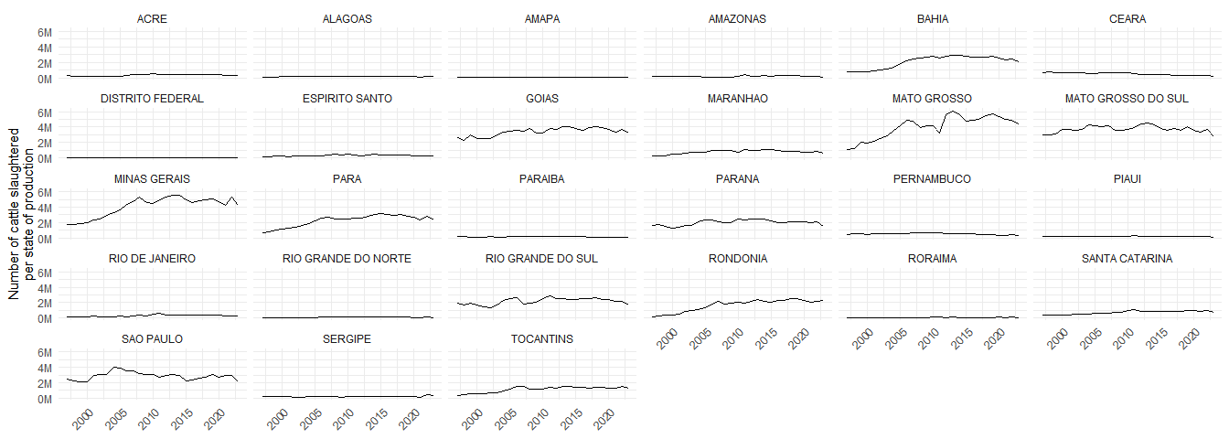
Calculate offtake rate
This is the number of heads * the slaughter rate, per state - plotted below.
# Define SR
# ... note I limit the calculation to 2006 onwards
# ... since these are the production years used in SEI-PCS
sr_df <-
  ppm %>%
  filter(YEAR >= 2006) %>%
  group_by(STATE, YEAR) %>%
  summarise(
    HERD_SIZE = sum(NUM_HEAD)
    ) %>%
  ungroup() %>%
  inner_join(slaughter, by = c("YEAR", "STATE")) %>%
  mutate(SR = NUM_HEAD_PER_STATE_OF_PRODUCTION / HERD_SIZE)


# Visualise data
sr_df %>%
  group_by(STATE) %>%
  summarise(MEAN = mean(SR),
            MEDIAN = median(SR),
            MIN = min(SR),
            MAX = max(SR)) %>%
  ungroup() %>%
  mutate(OUTLIER = ifelse(MEDIAN > 0.251, T, F)) %>%
  ggplot(aes(STATE, MEDIAN, col = OUTLIER)) +
  geom_point() +
  geom_errorbar(aes(ymin = MIN, ymax = MAX), width = 0, size = 0.5) +
  scale_y_continuous(limits = c(0, 1) ) +
  coord_flip() +
  ylab("Slaughter rate")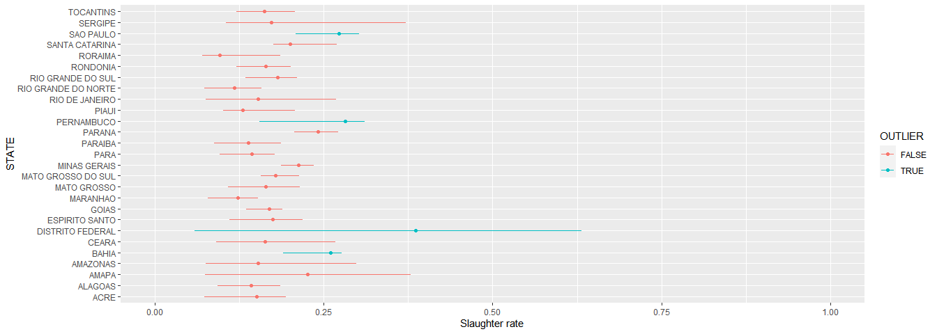
outlier_states <-
  sr_df %>%
  group_by(STATE) %>%
  summarise(MEDIAN = median(SR)) %>%
  ungroup() %>%
  filter(MEDIAN > 0.251) %>%
  pull(STATE)
national_median <- median(sr_df$SR)
I don’t believe the values in blue - they are too high (i.e. > 0.25: PE, AP, DF, BA), nor do I believe SP which is too low.
Below we correct for these outliers. For PE, AP, DF, and BA we set them to the national median (0.1726267), and for SP we use a state-specific value, based on other data sources (described below).
Note: I also considered using a time-invariant slaughter rate (i.e. one per state, not per state/year), but decided against it. Comparing the two methods (the alternative is commented out code), there is only a small difference, plus this way we keep more information and it allows SRs to increase over time, as they do in some states (e.g. RS?), see below:
sr_df %>%
  filter(YEAR > 2005,
         !STATE %in% outlier_states ) %>%
  ggplot(aes(YEAR, SR)) +
  # facet_wrap(~STATE, scale = "free_y") +
  facet_wrap(~STATE) +
  geom_line() +
  theme_minimal() +
  theme(axis.text.x = element_text(angle = 45, hjust = 1))
# I don't believe the outlier values > 0.25
# ... set these to nationwide average
# I also increase the SP production
# ... based on IEA data: http://www.iea.sp.gov.br/out/TerTexto.php?codTexto=14514
# ... otherwise production is too low.
sr_df <- sr_df %>%
  mutate(SR = case_when(STATE == "SAO PAULO" ~ 0.4072,
                        STATE %in% outlier_states ~ national_median,
                        TRUE ~ SR))  %>%
  select(STATE, YEAR, SR)

# The commented out code would be to produce a time-invariant estimate of the SR
# ... i.e. one value per state, not per state/yr
# sr_df <- sr_df %>%
#   mutate(SR = case_when(STATE == "SAO PAULO" ~ 0.4072,
#                         STATE %in% outlier_states ~ national_median,
#                         TRUE ~ SR))  %>%
#   group_by(STATE) %>%
#   summarise(SR = median(SR)) %>%
#   ungroup()
Carcass weights
# Carcass weights
# ... get mean per state/year (from the data which are originally trimestral)
cw <-
  s3read_using(
    object = "brazil/production/statistics/ibge/cattle/carcass_weights/2024-01-31-STATE_CARCASS_WEIGHTS.csv",
    bucket = "trase-storage",
    FUN = read_delim,
    opts = c("check_region" = T),
    delim = ";"
    )
Calculate cattle production
Per municipality per year, including offal - the latter calculated at 6.3% of the live cattle weight (450kg), based on FAO conversion coefficients.
# Calculate production
# ... CW_PRODUCTION_TONS = carcass + offal
# ... offal figure (6.3% of 450 kg cattle comes from Brazil-specific FAO coefficients).
cp <-
  inner_join(ppm, sr_df, by = c("STATE", "YEAR")) %>%
  left_join(cw, by = c("STATE" = "STATE_NAME", "YEAR")) %>%
  filter(YEAR %in% unique(cw$YEAR)) %>%
  mutate(
    NUM_HEAD_SLAUGHTERED = NUM_HEAD * SR,
    CW_PRODUCTION_TONS = NUM_HEAD_SLAUGHTERED * CARCASS_WEIGHT_PER_ANIMAL_KG / 1000 + (NUM_HEAD_SLAUGHTERED * 0.45 * 0.063)
    ) %>%
  select(GEOCODE, STATE, YEAR, CW_PRODUCTION_TONS)

# The commented out code would be to produce a time-invariant estimate of the SR
# ... i.e. one value per state, not per state/yr
# cp <-
#   full_join(ppm, sr_df, by = "STATE") %>%
#   left_join(cw, by = c("STATE" = "STATE_NAME", "YEAR")) %>%
#   filter(YEAR %in% unique(cw$YEAR)) %>%
#   mutate(
#     NUM_HEAD_SLAUGHTERED = NUM_HEAD * SR,
#     CW_PRODUCTION_TONS = NUM_HEAD_SLAUGHTERED * CARCASS_WEIGHT_PER_ANIMAL_KG / 1000 + (NUM_HEAD_SLAUGHTERED * 0.45 * 0.063)
#     ) %>%
#   select(GEOCODE, STATE, YEAR, CW_PRODUCTION_TONS)
stopifnot(!any(is.na(cp$CW_PRODUCTION_TONS)))
For the year 2019, visualise the production per municipality. Note: the scale is obviously skewed by large municipalities.
# Load spatial data
munis <-
  s3read_using(
    object = "brazil/spatial/BOUNDARIES/ibge/old/boundaries municipalities/MUNICIPALITIES_BRA.geojson",
    FUN = read_sf,
    bucket = "trase-storage",
    opts = c("check_region" = T)
  )
brazil <- st_union(munis)
munis_to_plot <- inner_join(munis,  cp %>% filter(YEAR == 2021), by = "GEOCODE")


# Visualise
ggplot() +
  geom_sf(data = brazil, fill = 'lightgrey') +
  geom_sf(data = munis_to_plot, aes(fill = CW_PRODUCTION_TONS), col = NA) +
  theme(axis.text = element_blank()) +
  coord_sf(datum = NA) +
  scale_fill_viridis(option="magma",
                     name = bquote('Tons/yr'),
                     na.value="white",
                     direction = -1) +
  labs(title = "Municipal cattle production (carcass tons/year)",
        subtitle = "For 2021")
Cattle lifecycle calculation
Sum production across the 5-yr cattle lifecycle.
# For each year, calculate the liveweight production over the previous 5 years
cp_5yr <-
  cp %>%
  # select(GEOCODE, YEAR, CW_PRODUCTION_TONS)  %>%
  group_by(GEOCODE) %>%
  arrange(YEAR) %>%
  mutate(CW_PRODUCTION_TONS_5_YR =
           CW_PRODUCTION_TONS +
           lag(CW_PRODUCTION_TONS, n = 1L) +
           lag(CW_PRODUCTION_TONS, n = 2L) +
           lag(CW_PRODUCTION_TONS, n = 3L) +
           lag(CW_PRODUCTION_TONS, n = 4L)) %>%
  ungroup()


# Check the lag worked OK
# ... this should really br run for multiple municipalities, not just one.
check_5_yr <-
  cp_5yr %>%
  filter(GEOCODE == "1507300",
         YEAR == 2017) %>%
  pull(CW_PRODUCTION_TONS_5_YR)
check_5_yr_manual <-
  cp_5yr %>%
  filter(GEOCODE == "1507300",
         YEAR %in% c(2013:2017)) %>%
  pull(CW_PRODUCTION_TONS) %>%
  sum()
if(
  !isTRUE(
    all.equal(
      check_5_yr,
      check_5_yr_manual,
      tolerance = 0.0001
    )
  )
){stop("Error in lag - go back and check")}
Visualise the 5-yr sum production data
# Visualise
munis_to_plot <- inner_join(munis, cp_5yr %>% filter(YEAR == 2019), by = "GEOCODE")
ggplot() +
  geom_sf(data = brazil, fill = 'lightgrey') +
  geom_sf(data = munis_to_plot, aes(fill = CW_PRODUCTION_TONS_5_YR), col = NA) +
  theme_minimal() +
  theme(axis.text = element_blank()) +
  coord_sf(datum = NA) +
  scale_fill_viridis(option="magma",
                     name = bquote('Tons/5yr lifecycle'),
                     na.value="white",
                     direction = -1) +
  labs(title = "Life-cycle cattle production (carcass tons/5-years)",
        subtitle = "For 2019")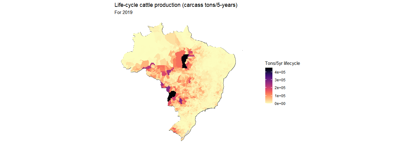
Export data
# Export the 5-yr data
s3write_using(
x = cp_5yr,
object = "brazil/production/statistics/ibge/beef/out/2024-01-31-CATTLE_PRODUCTION_5_YR.csv",
bucket = "trase-storage",
FUN = write_delim,
opts = c("check_region" = T),
delim = ";"
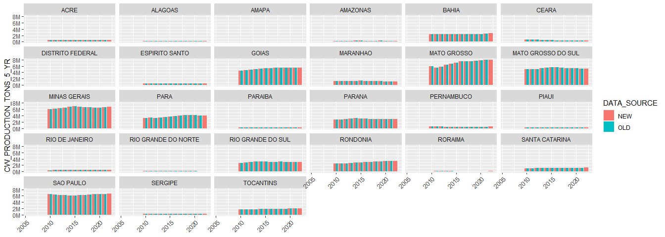
)Comparison with previous data
Looks good.